Stat 511 Solutions to Exam I Spring 2000
There may be more than one way to correctly answer a question, or several ways to describe the same answer. Not all of the possible correct answers may be listed here.
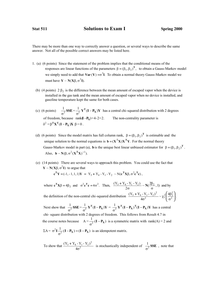
1. (a) (6 points) Since the statement of the problem implies that the conditional means of the
responses are linear functions of the parameters
β ==
(
β
1
,
β
2
)
T
, to obtain a Gauss-Markov model
we simply need to add that Var ( Y )
== σ 2
I .
To obtain a normal theory Gauss-Markov model we
must have Y ~ N ( X
β
,
σ 2
I ).
(b) (4 points) 2
β
2
is the difference between the mean amount of escaped vapor when the device is installed in the gas tank and the mean amount of escaped vapor when no device is installed, and gasoline temperature kept the same for both cases.
(c) (6 points)
σ
1
2
SSE =
of freedom, because
σ
1
2
Y
T rank( I
−−
( I
P
X
−−
)
P
X
= 4 -
) Y
2 =
has a central chi-squared distribution with 2 degrees
2.
The non-centrality parameter is
δ 2
=
β T
X
T
( I
−−
P
X
) X
β
= 0 .
(d) (6 points) Since the model matrix has full column rank,
β ==
(
β
1
,
β
2
)
T
is estimable and the
unique solution to the normal equations is b
==
( X
T
X ) X
T
Y .
For the normal theory
Gauss-Markov model in part (a), b is the unique best linear unbiased estimator for
β ==
(
β
1
Also, b ~ N (
β
,
σ 2
( X
T
X )
−−
1
).
,
β
2
)
T
.
(e) (14 points) There are several ways to approach this problem. You could use the fact that
Y ~ N ( X
β
,
σ 2
I ) to argue that c
T
Y
==
(-1, 1, 1, 1) Y
==
Y
3
++
Y
4
Y
1
Y
2
~ N( c
T
X
β
,
σ 2 c
T c ) ,
where c
T
X
β ==
4
β
2 and
σ 2 c
T c
==
4
σ 2
.
Then,
(Y
3
++
Y
4
Y
2
σ
1
Y
2
)
~ N (
2
β
σ
2
the definition of the non-central chi-squared distribution
, 1 ) and by
(Y
3
++
Y
4
Y
1
Y
2
4
σ 2
)
2
~
χ 2
1


4
β
σ 2
2
2
Next show that
1
σ 2
SSE =
1
σ 2
Y
T
( I
−−
P
X
) Y =
1
σ 2
Y
T
( I
−−
P
X
)
T
( I
−−
P
X
) Y has a central
chi- square distribution with 2 degrees of freedom. This follows from Result 4.7 in
the course notes because A =
σ
1
2
( I
−−
P
X
)
Σ
A =
σ 2
I
1
σ 2
( I
−−
P
X
)
==
( I
−−
P
X
)
is a symmetric matrix with rank(A) = 2 and
is an idempotent matrix.
To show that
(Y
3
++
Y
4
Y
1
Y
2
4
σ 2
)
2
1
is stochastically independent of
σ 2
SSE , note that

 .

(Y
3
++
Y
4
Y
1
Y
2
4
σ 2
)
2 is a function only of
1
σ 2
SSE =
σ
1
2
Y
T
( I
−−
P
X
)
T
( I
−−
P
X
) Y
(-1, 1, 1, 1) Y
== is a function only of
Y
( I
3
++
Y
4
−−
P
X
)
Y
1
Y
2
Y and
. Then,
(Y
3
++
Y
4
Y
1
4
σ 2
Y
2
)
2 is stochastically independent of
independent of the residual vector ( I
−−
P
X
) Y . Since
σ 2
Y
1
SSE if (-1, 1, 1, 1) Y is has a multivariate normal distribution,
it follows that

1


1 1
I P
X
1


 Y has a multivariate normal distribution. Then, to show that
(-1, 1, 1, 1) Y is independent of ( I
−−
P
X
) Y , we only need to show that the quantities are
uncorrelated. Here,
Cov (( -1, 1, 1, 1) Y , ( I
−−
P
X
) Y )
==
(-1, 1, 1, 1)(
σ 2
I )( I
−−
P
X
)
== σ 2
(-1, 1, 1, 1)( I
−−
P
X
)
==
(0,0,0,0)
because (-1, 1, 1, 1)
T is a column of X . Consequently,
F
==
(Y
3
++
Y
4
-
4
σ
Y
1
2
SSE
2
σ 2
Y
2
)
2
==
(Y
3
++
Y
4
Y
2SSE
1
Y
2
)
2
has an F-distribution with (1,2) degrees of freedom and non-centrality parameter 4
β 2
2
/
σ 2
because it is the ratio of a non-central chi-square random variable, divided by its degrees of
freedom, over an independent central chi-square random variable divided by its degrees of
freedom. This is the definition of a non-central F random variable.
Alternatively, you could note that
(Y
3
++
Y
4
Y
1
Y
2
4
σ 2
)
2
==
( c
T
( c
Y )( c
T c )
σ
T
2
Y )
==
Y
T c ( c
σ
T c ) c
2
T
Y
==
Y
T
A
1
Y ,
and apply Result 4.7 to this quadratic form and use Result 4.8 to show that this quadratic
form is independent of SSE.
(f) (4 points) Since the non-centrality parameter for the F-statistic in part (e) is 4
β 2
2
/
σ 2 hypothesis is H
0
:
β
2
==
0 and the alternative is H a
:
β
2
≠≠
0.
, the null
(g) (10 points) Since any linear function of a normally distributed random vector has a normal distribution, it follows that a
T
Y ~ N( a
T
X
β
,
σ 2 a
T a ).
Then, a
T
Y
σ 2 a
T a
~ N( a
T
X
β
σ 2 a
T a
, 1) and it follows that
( a
T
Y )
2
σ 2 a
T a
~
χ 2
1


( a
T
X
β
)
2
σ 2 a
T a

 .
In part (e) we also showed that
1
σ 2
1
SSE =
σ 2
Y
T
( I
−−
P
X
) Y has a central chi- square distribution
with 2 degrees of freedom. Then, the statistic shown in this part has an F-distribution if
( a
T
Y )
2
σ 2 a
T a is independent of
1
σ 2
1
SSE =
σ 2
Y
T
( I
−−
P
X
) Y . Using the argument from part (e), this

is true if Cov ( a
T
Y , ( I
−−
P
X
) Y )
== a
T
(
σ 2
I )( I
−−
P
X
)
== σ 2 a
T
( I
−−
P
X
)
==
(0,0,0,0) . Hence, the statistic
has an F-distribution if a is in the space spanned by the columns of X, that is, if a
== a






0

1
0
1




 ++ b

-




-
1

1



1
1 


==





 a a
b
++
b b b 





for some constants a and b where either a
≠≠
0 or b
≠≠
0.
2. (a) (6 points)
γ
1
is the mean corn yield for variety A grown with nitrogen applied at 150lb/a.
100
δ
1 is the difference between mean yields for nitrogen applied at 200lb/a and 100lb/a
for either variety A or variety B.
(b) (6 points) Since the model matrix has full column rank, any linear combination of the parameters is estimable. Hence, both (i) and (ii) are estimable.
(c) (4 points)
µ ++ α
1
is estimable because E[ (Y
1
+ Y
2
+ Y
3
)/3) ] =
µ ++ α
1
.
(d) (6 points) Delete the third row and the third column of X
T
X . Invert the remaining 4x4 matrix.
Fill in zeros for the third row and third column of the generalized inverse. Alternatively you could use the spectral or singular value decomposition of X
T
X to obtain a generalized inverse.
(e) (8 points) First show that unbiased estimator for (0,
α
1
-
α
2
1, -
is estimable. Then,
1, 0, 0)
β == α
1
−− α
2
(0, 1, 1, 0, 0) b is the unique best linear
. Furthermore, since the random errors are independent N ( 0 ,
σ 2
) random variables, c
T b ~ N (
α
1
-
α
2
,
σ 2 c
T
( X
T
X )
−− c ), where c
T ==
(0, 1, 1, 0, 0).
(f) (6 points) Yes, because the columns of the model matrices span the same linear space. Let
W
==
[ w
1
| w
2
| w
3
| w
4
] denote the model matrix for Model 1, and let X
==
[ x
1
| x
2
| x
3
| x
4
| x
5
] denote the model matrix for Model 2. Then, and w
4
== x
5
==
(
2500 (
3 w
4 x
5
++
/ 2500 ) 2 w
1
2 x
2
++
2 x
3
) /
-
3
2
.
w
2
.
Also, w
1 x
==
2 x
2
==
, w
1 w
, x
3
2
== x
==
3
, w
2 w
3
, x
1
==
== w
50 x
4
1
,
++ w and
2
, x
4
== w
3
/ 50 ,
(g) (6 points) Since the quantity is estimable, the unique b.l.u.e. for the mean yield of variety 1 using
120 lb/a of nitrogen is c
T b
==
( 1, 0, 30, 900) b ~ N ( c
T γγ
,
σ 2 c
T
( W
T
W )
−− c ), where b
==
( W
T
W )
−−
W
T
Y is a solution to the normal equations. Using the MSE from the ANOVA to estimate
σ 2
, a 95% prediction interval is
( 1, 0, 30, 900) b
±±
t
2,.025
MSE ( 1
++ c
T
( W
T
W )
−− c )
where t
2,.025
is the upper 0.025 percentile of a central t-distribution with 2 degrees of freedom.

(h) (8 points) Write the null hypothesis as H
0
: C
γ == 

 1 -
0
1
0
0 0
0 1 








γ
γ
δ
δ
1
2
1
2






==



0
0 


, and let b
==
( W
T
W )
−−
W
T
Y be any solution to the normal equations. The null hypothesis would be rejected if b
T
C
T
( C
T
( W
T
W)
−−
C)
−−
1
C b
F
== 2
MSE
exceeds the upper
α
percentile of a central F-distribution with (2,2) degrees of freedom, where
α
is the type I error level of the test.
The exam scores (out of 100 points) are presented as a stem-leaf display:
90 | 8
90 | 0 1
80 | 7 8 9
80 | 0 3
70 | 5 5 5 5 5 7 8
70 | 0 1 2 3 3 4
60 | 7 7 8 9
60 | 0 0 1 1 3
50 | 6 7 7 7 7 8 8 8 8 9
50 | 0 1 4 4
40 | 5 6 8 9
40 | 0 2 3
30 | 9 9
30 | 2
20 | 5 9
A point value should be shown for the credit awarded for each part of your exam, corresponding
to the point values listed above. If your answer failed to earn any credit, a zero should be shown.
If no point value is shown for some part of your exam, show your exam to the instructor. Also,
check if the total points recorded on the last page of your exam is correct.