© 2002 by The Arizona Board of Regents
for The University of Arizona.
All rights reserved.
Business Mathematics II
SOLUTIONS
FOR STUDY GUIDE 2
The following questions examine parts of the material which will be covered on Test 2.
Questions 1-8 refer to the continuous random variable, X, whose p.d.f. and c.d.f. are given
below.
0 if x  0
 2
x
FX ( x )  
if 0  x  2
 4

1 if 2  x
0 if x  0
x
f X ( x)  
if 0  x  2
2
0 if 2  x

1. Is fX or FX the probability density function of X?
Solution. The probability density function of X is fX.
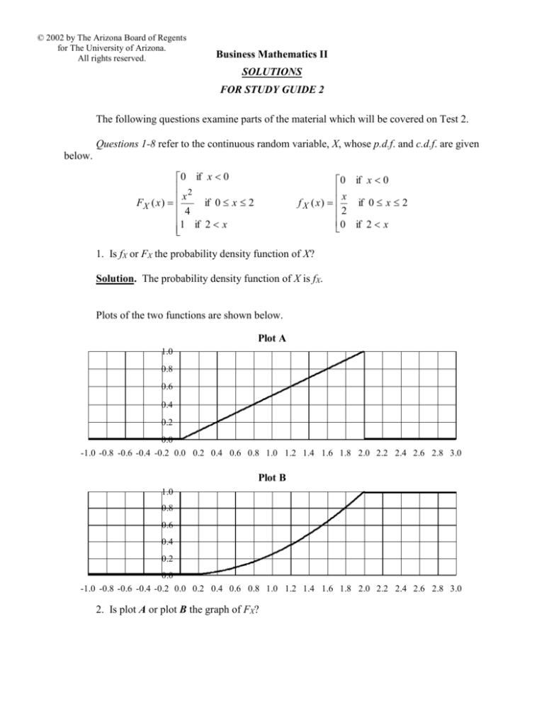
Plots of the two functions are shown below.
Plot A
1.0
0.8
0.6
0.4
0.2
0.0
-1.0 -0.8 -0.6 -0.4 -0.2 0.0 0.2 0.4 0.6 0.8 1.0 1.2 1.4 1.6 1.8 2.0 2.2 2.4 2.6 2.8 3.0
Plot B
1.0
0.8
0.6
0.4
0.2
0.0
-1.0 -0.8 -0.6 -0.4 -0.2 0.0 0.2 0.4 0.6 0.8 1.0 1.2 1.4 1.6 1.8 2.0 2.2 2.4 2.6 2.8 3.0
2. Is plot A or plot B the graph of FX?
- Solutions for Study Guide for Business Mathematics II, Test 2: page 2 -
Solution. Plot B the graph of FX?
3. On the plot of fX , shade the region whose area corresponds to P(0.8  X  1.6).
Solution.
Plot A
1.0
0.8
0.6
0.4
0.2
0.0
-1.0 -0.8 -0.6 -0.4 -0.2 0.0 0.2 0.4 0.6 0.8 1.0 1.2 1.4 1.6 1.8 2.0 2.2 2.4 2.6 2.8 3.0
4. Use the region from Question 3 to estimate P(0.8  X  1.6). Note that the area of
each grid square is 0.04 square units.
Solution. P(0.8  X  1.6) is approximately equal to 0.5.
5. Use the formula for the c.d.f. of X to compute P(0.8  X  1.6) exactly.
Solution. P(0.8  X  1.6) = FX(1.6)  FX(0.8) = 1.62/4  0.82/4 = 0.48.
6. Set up and evaluate an integral that computes P(0.8  X  1.6). Round your answer to
three decimal places.
1.6
Solution. P (0.8  X  1.6) 

0 .8
x
dx Using Integrating.xls, we find a value of 0.480
2
for the integral.
7. Set up and evaluate an integral that computes the expected value, E(X), of X. Round
your answer to three decimal places.
2
x
Solution. E ( X )  x    dx Using Integrating.xls, we find a value of 1.333 for the
2

0
integral.
- Solutions for Study Guide for Business Mathematics II, Test 2: page 3 -
8. Set up and evaluate an integral, that computes the variance, V(X), of X. Round your
answer to three decimal places. (You will need to use the value for X that you computed in
Question 7.
2
Solution. V ( X ) 
2 x


x


   dx
X

2
0
Using Integrating.xls, we find a value of 0.222
for the integral.
Questions 9-11 refer to the finite random variable X, whose p.m.f. is given below.
x
fX(x)
0
0.2
1
0.3
2
0.3
4
0.1
8
0.1
9. Compute the mean, X, of X.
 x  f X ( x)  0  0.2  1  0.3  2  0.3  4  0.1  8  0.1  2.1
Solution.  X 
all possible x
10. Compute the variance, V(X), of X.
Solution. V ( X ) 
 x   X 2  f X ( x)
all possible x
 (0  2.1) 2  0.2  (1  2.1) 2  0.3  ( 2  2.1) 2  0.3
 ( 4  2.1) 2  0.1  (8  2.1) 2  0.1
 0.882  0.363  0.003  0.361  3.481  5.09
11. Compute the standard deviation, X, of X. Round your answer to 3 decimal places.
Solution.  X  V ( X )  5.09  2.256
Questions 12-16 refer to the random variable X which gives the number of customers
who visit your business in a given day. You know that the parameters of X are X = 30 and X =
6, but you do not know the p.d.f. or the c.d.f. for X. Let x be the random variable that is the
mean of a random sample of size n = 80 days.
12.   ?
x
Solution.  x   X  30.
- Solutions for Study Guide for Business Mathematics II, Test 2: page 4 -
13. V ( x )  ?
Solution. V ( x )  V ( X ) / 80  62 / 80  0.45.
14.   ?
x
Solution.  x   X / n  6 / 80  0.671.
15. Give a formula for the random variable, S, that is the standardization of x .
Solution. S 
x  x

x
x  30
.
6 / 80
16. What is the approximate distribution of S?
Solution. S has a c.d.f. which is approximately standard normal.
Questions 17-19 refer to the following sample of size n = 6 taken for the values of a
random variable.
10.3, 12.4, 8.9, 10.3, 9.0, 11.8
17. Compute the sample mean, x .
Solution. x 
1

n
x

all possible x
1
62.7
 10.3  12.4  8.9  10.3  9.0  11.8 
 10.45
6
6
18. Compute the sample variance, s2.
Solution. s 2 
1

n 1

 x  x 
2
all possible x
1
 (10.3  10.45) 2  (12.4  10.45) 2    (11.8  10.45) 2
5
10.175

 2.035
5


- Solutions for Study Guide for Business Mathematics II, Test 2: page 5 -
19. Compute the sample standard deviation, s. Round your answer to 3 decimal places.
2
Solution. s  s  2.035  1.427
Questions 20-24 refer to the following plots of p.d.f.’s.
a.
b.
0.6
0.5
0.4
0.3
0.2
0.1
0
-1
c.
0
1
2
3
4
-4
e.
-3
-1
1
3
5
0.15
0.1
0.05
0
0
4
8
12
16
f.
0.15
0.1
0.05
0
-10
-5
d.
0.6
0.5
0.4
0.3
0.2
0.1
0
0.5
0.4
0.3
0.2
0.1
0
-5
0
5
10
15
20
-4
0
4
8
12
16
20
0.5
0.4
0.3
0.2
0.1
0
-1
1
3
5
7
9
11
20. Which one could correspond to a standard normal random variable?
Solution. b.
21. Which one could correspond to a uniform random variable?
Solution. a.
22. Which one could correspond to an exponential random variable?
Solution. c.
23. Which ones could not possibly correspond to a normal random variable? (There
might be more than one.)
Solution. a and c.
- Solutions for Study Guide for Business Mathematics II, Test 2: page 6 -
24. Which one could correspond to a normal random variable with X =5 and X = 3?
Solution. e.
Questions 25 and 26 refer to the following situation. Fifteen (15) companies all bid on
oil leases. The following data is a small part of the records on past bids. All monetary amounts
are in millions of dollars.
Leases
Proven Value
$103.3
$109.5
$98.7
Signals
Company 1
Company 2
$99.0
$102.4
$91.7
$111.3
$105.8
$113.7
25. Compute the mean error in the signals.
Solution. The six errors are shown below.
Errors
$4.3
$0.9
$1.8
$17.8
$7.1
$15.0
The mean error is ($4.3  $0.9  $17.8 + $1.8 + $7.1 + $15.0)/6 = $0.15.
Let R be the continuous random variable giving the error in a geologist's estimate for the
value of a lease. Experience allows us to assume that R is normal, with R = 0 and R = 10
million dollars. Suppose that the 15 companies form 3 bidding rings of equal sizes. Let M be
the random variable giving the mean of the errors for a set of signals for the companies in one of
the bidding rings.
26. Compute the standard deviation, M, for M? Round your answer to 3 decimal places.
Solution. Since there are 3 rings of the same size, there are 5 companies in each ring and

M is the sample mean for n = 5, from R.  M  R
n
 10
5
 4.472
- Solutions for Study Guide for Business Mathematics II, Test 2: page 7 -
Questions 27-29 refer to the following situation. A normal random variable X gives the
number of ounces of soda in a randomly selected can from a given canning plant. It is known
that the mean of X is close to 12 ounces and that X = 0.4 ounces. A plot of fX is shown below.
3.0
2.5
2.0
1.5
1.0
0.5
0.0
10.5
11.0
11.5
12.0
12.5
13.0
13.5
Let x be the mean of a random sample of size n = 4 soda cans.
27.  x  ?
Solution.  x 
X
n

0.4
 0.2
4
28. Sketch a graph of the probability density function for x on the above plot.
Solution.
3.0
2.5
2.0
1.5
1.0
0.5
0.0
10.5
11.0
11.5
12.0
12.5
13.0
13.5
29. Use standard deviations to explain why the mean of a sample of size n = 16 cans
would be likely to give a better estimate for X than would the mean of a sample of size n = 4
cans.
Solution. The standard deviation for the sample mean with a sample size of 16 is 0.4/4 =
0.1. At n = 16, the confidence intervals, for any given level of confidence, for X will be onehalf the width of those for a sample size of 4.
- Solutions for Study Guide for Business Mathematics II, Test 2: page 8 -
30. Let X be a normal random variable with X = 24 and X = 3.2. Fill in the information
that would be needed to have the Excel function Random Number Generation create random
values of X in Cells A1:F10.
Solution.
6
10
Normal
24
3.2
A1