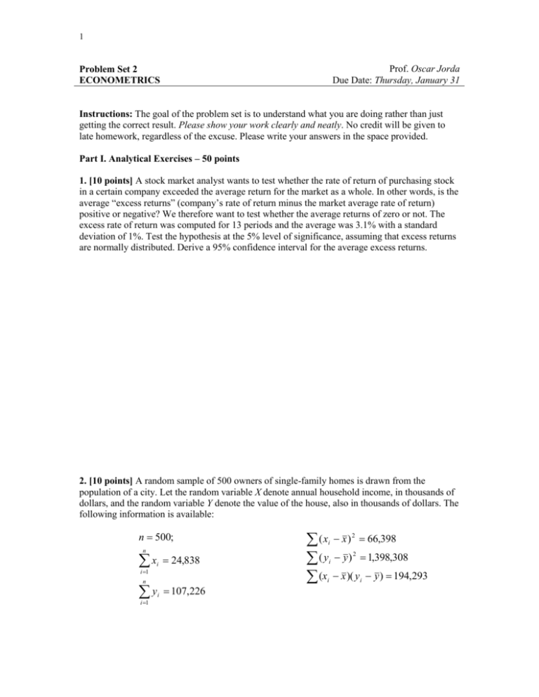
1
Prof. Oscar Jorda
Due Date: Thursday, January 31
Problem Set 2
ECONOMETRICS
Instructions: The goal of the problem set is to understand what you are doing rather than just
getting the correct result. Please show your work clearly and neatly. No credit will be given to
late homework, regardless of the excuse. Please write your answers in the space provided.
Part I. Analytical Exercises – 50 points
1. [10 points] A stock market analyst wants to test whether the rate of return of purchasing stock
in a certain company exceeded the average return for the market as a whole. In other words, is the
average “excess returns” (company’s rate of return minus the market average rate of return)
positive or negative? We therefore want to test whether the average returns of zero or not. The
excess rate of return was computed for 13 periods and the average was 3.1% with a standard
deviation of 1%. Test the hypothesis at the 5% level of significance, assuming that excess returns
are normally distributed. Derive a 95% confidence interval for the average excess returns.
2. [10 points] A random sample of 500 owners of single-family homes is drawn from the
population of a city. Let the random variable X denote annual household income, in thousands of
dollars, and the random variable Y denote the value of the house, also in thousands of dollars. The
following information is available:
n  500;
n
x
i 1
i
i 1
2
i
2
i
i
n
y
 24,838
 ( x  x )  66,398
 ( y  y )  1,398,308
 (x  x )( y  y )  194,293
i
 107,226
i
2
(a) Compute the mean and standard deviation of the value of the houses and household income in
this sample.
(b) Compute the correlation between income and house value.
(c) Construct a 95% confidence interval for the mean value of houses. What assumptions do you
need to make to do this?
(d) Using a two-tailed test at the 0.01 level, test the hypothesis that the correlation between
income and house value is zero.
3. [10 points] Let X and Y represent the rates of return (in percent) on two stocks. You are told
that X ~ N(15,25) and Y ~ N(8,4) and that the correlation coefficient between the two rates of
return is –0.4. Suppose you want to hold the two stocks in your portfolio in equal proportion.
(a) What is the probability distribution of the return in your portfolio?
(b) Suppose you want to maximize your return. Does this portfolio accomplish that goal?
(c) Suppose you want to minimize your exposure (risk). Calculate the asset allocation between
assets X and Y that would accomplish this goal?
3
4. [10 points] Let X ~ N(, 2). A random sample of three observations was obtained from this
population. Consider the following estimators of :
ˆ 1 
X1  X 2  X 3
3
ˆ 2 
X1 X 2 X 3


6
3
2
(a) Is ̂ 1 an unbiased estimator of ? Is ̂ 2 ? Demonstrate.
(b) Calculate the variance of these estimators.
(c) Based on your answers in parts (a) and (b), which estimator would you prefer? Explain your
answer using unbiasedness, consistency and efficiency arguments.
4
5. [10 points] True or false? Explain.
(a) The null hypothesis says the effect is zero.
(b) The alternative hypothesis says that nothing is going on besides chance variation.
(c) A hypothesis test tells you whether or not you have a useful sample.
(d) A significance level tells you how important the null hypothesis is.
(e) The p-value will tell you at what level of significance you can reject the null hypothesis.
(f) Calculation of p-values is useless for significance tests.
(g) It is always better to use a significance level of 0.01 than a level of 0.05.
(h) If the p-value is 0.45, the null hypothesis looks plausible.
(i) With small samples and large , quite large differences may not be statistically significant but
may be real and of great practical importance.
(j)The conclusions from the data cannot be summarized by the p-value. Conclusions should
always have a practical meaning in terms of the problem at hand.
(k) The power of a test at the null hypothesis is equal to the significance level.
Part II. Empirical Questions – 50 points
The data for this exercise is contained in the excel file “salary.XLS.” It contains 93 observations
on employees for a Chicago Bank during the period 1969-1971. In particular, the variable
“salary” refers to the starting salary, “education” refers to years of education, “experience” refers
to the number of months of previous work experience, “seniority” refers to the number of months
the person has been working at the current job with the bank, and “gender” takes the value of one
for males and 0 for females.
You will need to import the data into EViews. This can be easily accomplished by opening a new
workfile. Select the option corresponding to undated or irregular observations and a range that
5
goes from 1 to 93. Then from the “procs” button, select the import option, and the “excel” option
thereafter. The rest is pretty straightforward.
Answer the following questions:
1. Give summary statistics for all variables in one table. Then, subsample according to gender and
report the summary statistics with an additional two tables. Next, select all the variables (make
sure to undo the subsampling condition) and compute their correlations and include this table
with the previous tables in the same page. Comment on all of these results, making particular
emphasis on whether you see any evidence of discrimination (nothing formal yet, just hunches).
Beware of the experience and seniority levels of each group.
2. Do a formal test of the null hypothesis that females are discriminated against at a 5%
confidence level. Do your results hold at a 1% confidence level? Consider now a test of the null
hypothesis that males earn $250 more than females on average at a 5% confidence level. Make
sure to report these tests in one page and in one paragraph report on the economic significance of
your tests (Is there gender bias in pay scales?). Hints: make sure you consider whether a onetailed test or a two-tailed test is appropriate.
3. Load data on the exchange rate between the U.S. dollar and the Japanese yen into EViews.
Select monthly frequency and select a data source that begins at least in 1980. You will need to
plot these data and compute summary statistics. Regarding the plot, make sure that you label
important economic dates (such as oil crises, or other political events) that may help explain some
of the long swings in these data. Make sure to label the graph appropriately, including title, units
of measurement, etc. Both the plot and the summary statistics should fit in one page.