KYIV SCHOOL OF ECONOMICS
Financial Econometrics (2nd part):
Introduction to Financial Time Series
May 2011
Instructor: Maksym Obrizan
# 2. This lecture:
(i) Very brief summary of ARCH-GARCH and
their shortcomings
(ii) A few more advanced models (TAR, MSA)
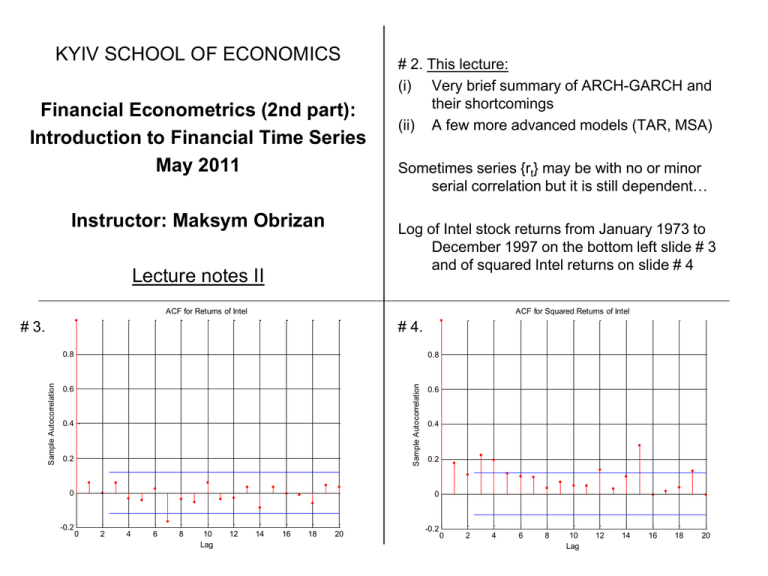
Sometimes series {rt} may be with no or minor
serial correlation but it is still dependent…
Log of Intel stock returns from January 1973 to
December 1997 on the bottom left slide # 3
and of squared Intel returns on slide # 4
Lecture notes II
ACF for Returns of Intel
ACF for Squared Returns of Intel
# 3.
# 4.
0.8
Sample Autocorrelation
Sample Autocorrelation
0.8
0.6
0.4
0.2
0
-0.2
0.6
0.4
0.2
0
0
2
4
6
8
10
Lag
12
14
16
18
20
-0.2
0
2
4
6
8
10
Lag
12
14
16
18
20
ACF for Modulus Returns of Intel
# 5.
# 6. Series are uncorrelated but dependent:
volatility models attempt to capture such
dependence
Sample Autocorrelation
0.8
0.6
Define shock or mean-corrected return
0.4
0.2
0
-0.2
0
2
4
6
8
10
Lag
12
14
16
18
# 7. Then ARCH(m) model assumes
20
# 8. Practical way of building an ARCH model
(i) Build an ARMA model for the return series
to remove any linear dependence in data
If the residual series indicates possible ARCH
effects – proceed to (ii) and (iii)
(ii)
In practice, the error term is assumed to follow
the standard normal of a standardized
Student-t distribution
Specify the ARCH order and perform
estimation
(iii) Check the fitted ARCH model for necessary
refinements
# 9. Fitting an ARCH Model:
# 10. Shortcomings of ARCH model
(i) Positive and negative shocks have the
same effects on volatility
Model Checking:
Obtain standardized shocks

(ii)
Use kurtosis, skewness and QQ-plot of to
check if normal distribution is applicable
MOTIVATION FOR TAR, MSA MODELS!
ARCH model is restrictive – parameters are
constrained by certain intervals for finite
moments etc
(iii) Sometimes not parsimonious models: use
GARCH
# 11. GARCH model:
# 12. NOTES
Then use Ljung-Box statistic on
to check the
adequacy of the mean equation and on
to check the validity of the volatility equation.
Weaknesses of GARCH model are similar to
those of ARCH: symmetric response to
negative and positive shocks etc
# 13. Application: daily log returns of IBM stock
from July 3, 1962 to December 31, 1999
# 14. In addition, the Ljung-Box statistics of the
standardized residuals is Q(10) = 11.31 (pvalue of 0.33) and of the squared
standardized residuals is Q(10) = 11.86 (pvalue of 0.29)
All the estimates (except the coefficient of rt-2)
are highly significant
# 15. The unconditional mean of rt in this model
is
while in the sample it is only 0.045.
What if the model is misspecified?
 Motivation for nonlinear models such as
TAR and MSA
# 16. Threshold Autoregressive (TAR) model
Simulated 2-regime TAR(1) series
6
# 17. Consider a simple two-regime TAR model
5
# 18.
4
3
2
1
0
-1
-2
-3
# 19. Observe that this model has coefficient -1.5
0
20
40
60
80
100
120
140
160
# 20. Model behavior depends on xt -1:
When it is negative then
However, despite this fact it is stationary and
geomertically ergodic if
When it is positive then
Ergodic theorem – statistical theorem showing
that the sample mean of xt converges to the
mean of xt
Question: Which regime will have more
observations?
180
200
# 21. In addition, TAR model has non-zero mean
even though the constant terms are zero
(think of an AR(m) model with zero constant
for a comparison)
# 22. AR(2)-TAR-GARCH(1,1) of IBM stock
Re-consider slide # 15 with AR(2)-GARCH(1,1)
model of IBM stock: the unconditional mean
of 0.065 overpredicted the sample mean of
0.045
Estimate AR(2)-TAR-GARCH(1,1) model and
refine it (remove insignificant term in
volatility equation)
# 23. Model fit
All coefficients are significant at 5%
The unconditional mean?
The Ljung-Box statistics applied to standardized
residuals does not indicate serial
correlations or conditional heteroscedasticity
# 24. NOTES:
# 25. Convenient to re-write TAR-GARCH(1,1):
# 26. Recall the integrated GARCH model
(IGARCH is a unit-root GARCH model)
For example, IGARCH(1,1) is defined as
The unconditional variance of at, and thus of rt, is
not defined
Meaning: Occasional level shifts in volatility?
IGARCH(1,1) with
is used in
RiskMetrics (Value at Risk calculating)
# 27. Thus, under nonpositive deviation the
volatility follows an IGARCH(1,1) model
without a drift
With positive deviation, the volatility has a
persistent parameter 0.046+0.885=0.931
which is <1 giving rise to GARCH(1,1)
Conclusion:
# 28. NOTES:
# 29. Markov Switching Model
# 30. Application to the US quarterly real GNP
# 31. Cont’d
# 32. Notes
# 33. Nonlinearity tests: Parametric tests
# 34. Apply F statistic
The RESET Test for a linear AR(p) model
with g and T-p-g degrees of freedom
Basic idea: if a linear AR(p) model is adequate
then a1 and a2 should be zero.
# 35. Nonlinearity tests: Nonparametric tests
Q-statistic of Squared Residuals
The null hypothesis of the statistic is
# 36. NOTES
# 37. Application to the US quarterly civilian
unemployment from 1948 to 1993 based on
Montgomery, Zarnowitz, Tsay and Tiao
(1998)
# 38. TAR model
# 39. MSA model
# 40. NOTES