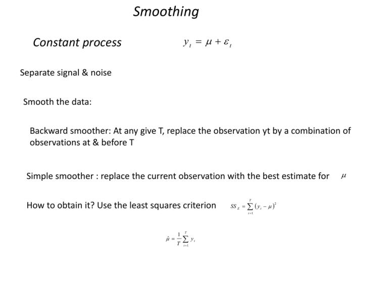
Smoothing
yt     t
Constant process
Separate signal & noise
Smooth the data:
Backward smoother: At any give T, replace the observation yt by a combination of
observations at & before T
Simple smoother : replace the current observation with the best estimate for
How to obtain it? Use the least squares criterion
T
SS E 
 y
t 1
ˆ 
1
T
T

t 1
yt
t
 
2

Not Constant process
Can we use ?
ˆ 
1
T
T

yt
t 1
this smoother accumulates more and more data points and gains some sort of inertia
So it cannot react to the change
Obviously, if the process change, earlier data do not carry the information about the it
Use a smoother that disregards the old values and reacts faster to the change
Simple moving average
Simple moving average
MT 
y T  y T 1    y T  N  1
N
Var ( M T ) 
1

N

N

yt
t  T  N 1
2
N
Choice of span N:
-If N small :reacts faster to the change
- large N:constant process
The moving averages will be autocorrelated since 2 successive moving averages contain the
same N-1 observations
k

 1 N , k  N
 k   0, k  N


First order exponential smoothing
Obtain a smoother that reacts faster to the change
Idea: give geometrically decreasing weights to the past observations
T 1

t
y T 1  y T   y T 1   y T  2    
2
T 1
y1
t0
However,
T 1

t
t0

1
T
1
Adjust the smoother , by multiplying
~
y T  1  
(1   )
1   
T
T 1
  t y T  t
t0
 1  
 y T
  y T 1   y T  2    
2
T 1
y1

Simple or first order
exponential smoother

2
T 1
~
y T  1    y T 1   T  y T  1     y T 1   y T  2    
y1
 1  
 1  
y
y
T
  1  
T
 ~
y T 1
 y T 1  
yT  2    
T 2
y1


First-order exponential smoothing:
linear combination of the current observation & the smoothed observation at the
previous time unit
~
y t  1    y T   ~
y T 1
~
y t   y T  (1   ) ~
y T 1
Discount factor  : weight on the last observation
(1   ) : weight on the smoothed value of the previous observations
The initial value
The initial value
2 commonly used estimates of
~
y 0  y1
~
y0  y
~
y0
~
y0
If the changes in the process are expected to occur early & fast
If the process at the beginning is constant
The value of 
As  gets closer to 1, & more emphasis is given in the last observations : the
smoothed values follow the original values more closely
  0:
~
yT  ~
y0
  1 : ~y T  y T
0 .1    0 .4
The smoothed values equal to a constant
The least smoothed version of the original time series
Values recommended
Choice of the smoothing constant:
1
Subjective: depending of willingness to have fast adaptivity or more
rigidity.
2
Choice advocated by Brown (inventor of the method): λ = 0.7
3
Objective: constant chosen to minimize the sum of squared forecast
errors
Use exponential smoothers for model estimation
General class of models
y t  f t ;     t
yt   0   t
e.g. constant process
T
SS E 
 y
t
 
2
t 1
If not all observations have equal influence on the sum : introduce weights that geometrically
decrease in time
T 1
SS
*
E

  y
T
T t
 0 
2
t0
Take the derivative
The solution
For large T
dSS
*
E
d 0
ˆ 0 
T 1
 2 
y
T t
 ˆ 0
t0
1
1
T
T 1
T

t
yT t
t0
T 1
t
ˆ 0  (1   )   y T  t  ~y T
t0

0
Second order exponential smoothing
Linear trend model
y t   0   1t   t
t
Uncorrelated with mean 0 & constant variance

2
Use single exponential smoothing: underestimate the actual values
Why?
 

t
E ~
y T   E    1    y T  t 
 t0


   1    E ( y T  t )
t
t0
Given
E  y t    0   1t

t
E ~
y T     1      0   1 (T  t ) 
t0


   0   1T   1      1  1    t
t
t
t0
t0
1 
E ~
y T     0   1T  
1

 E  yT  
1 

1
bias
Simple exponential smoother:biased
estimate for the linear trend model
Solutions:
a) Use a large value 
  1:
1 

 0
Smoothed values very close to the observed: fails to
satisfactorily smooth the data
b) Use a method based on adaptive updating of the
discount factor 
c) Use second order exponential smoothing
Second order exponential smoothing
Apply simple exponential smoothing on
~y
T
(2)
(1 )
(2)
~
y T  ~
y T  (1   ) ~
y T 1
(1 )
(2)
yˆ T  2 ~
yT  ~
yT
Unbiased estimate of yT
2 main issues: choice of initial values for the smoothers& the discount factors
Initial values
1  ˆ
(1 )
~
y 0  ˆ 0 , 0 
 1, 0

1   ˆ
2
~
y 0  ˆ 0 , 0  2 
  1, 0
  
Estimate parameters
through least squares
Holt’s Method
Divide time series into Level and Trend
Lt =λyt +(1−α)(Lt−1+Tt−1)
Tt =β(Lt +Lt-1 )+(1−β)Tt-1
Ft+1=Lt+Tt
yt = actual value in time t
λ = constant-process smoothing constant
β = trend-smoothing constant
Lt = smoothed constant-process value for period t
Tt = smoothed trend value for period t
F
= forecast value for period t + 1
t = current time period
Use exponential smoothers for forecasting
At time T, we wish to forecast observation at time T+1, or at time
yˆ T  T 
T +t
  step  ahead forecast
Constant Process
yt   0   t
Can be estimated by the first-order exponential
smoother
yˆ T   (T )  ~
yT
Forecast :
At time T+1
0
yˆ T 1   y T 1  1    ~
yT
yˆ T 1   y T 1  1    yˆ T  (T )
yˆ T 1 (T )  yˆ T (1)    y T 1  yˆ T 1
 yˆ T (1)   eT (1)
e T (1)  y T  1  yˆ T  1 (T )
One-step-ahead forecast error
yˆ T 1 (T )  yˆ T (1)    y T 1  yˆ T 1
 yˆ T (1)   eT (1)
Our forecast for the next observation is our previous forecast for the
current observation plus a fraction of the forecast error we made in
forecasting the current observation
Choice of 
Sum of the squared one-step-ahead forecast errors
SS E   
T
 e 1
2
t 1
t 1
Calculate for various values of

Pick the one that gives the smallest sum of squared forecast errors
Prediction Intervals
Constant process
~
y T  Z a ˆ e
2
first-order exponential smoother
~y
T
Za
2
ˆ e
100(1-a/2) percentile of the standard normal distribution
Estimate of the standard deviation of the forecast errors
Linear Trend Process
yˆ T  T 
  step  ahead forecast
yˆ T   T   ˆ 0 ,T  ˆ1 ,T T  

 ˆ 0 ,T  ˆ1,T T  ˆ1,T 
 yˆ T  ˆ1 ,T 
In terms of the exponential smoothers
(1 )
(2)
yˆ T      2 ~y T  ~y T   

1 
 ~y
(1 )
T
 2 ~y T
(2)




 (1 ) 
 (2)
 2 
  ~y T   1 
  ~y T
1  
1  


Parameter Estimates
æ
ö
è
ø
b0,T +1 = l (1+ l ) yT +1 + (1- l ) ç b0,T + b1,T ÷
2
b1,T +1 =
l
(b
2-l
0,T +1
)
- b0,T +
2 (1- l )
b1,T
(2 - l )
100(1-α/2) prediction intervals for any lead time τ
æ
ö
æ
ö
l
l
c
t ÷ yT(1) - ç1+
t ÷ yT(2) ± Za /2 t s e
ç2 +
è
è 1- l ø
1- l ø
c1
ci2 = 1+
l é
10 -14 l + 5l 2 ) + 2il ( 4 - 3l ) + 2i 2 l 2 ùû
3 ë(
(2 - l )
Estimation of the variance of the forecast errors, σe2
Assumptions: model correct & constant in time
Apply the model to the historic data & obtain the forecast errors
1 T 2
s = å et (1)
T t=1
2
e
=
2
1 T
yt+1 - yt+1 ( t ))
(
å
T t=1
Update the variance of the forecast errors when have more data
2
s e,T+1
=
2
s e,T+1
=
1
2
Ts e,T
+ eT2+1 (1))
(
T +1
T
1
eTt2 (t ))
å
(
T - t +1 t=t
Define mean absolute deviation Δ
(
D = E e - E ( e)
)
Assuming that the model is correct
DT = d eT (1) + (1- d ) DT -1
s e,T = 1.25DT
Model assessment
Check if the forecast errors are uncorrelated
Sample autocorrelation function of the forecast errors
T -1
åéëe (1) - e ùûéëe (1) - e ùû
t
rk =
t=k
t-k
T -1
åéëe (1) - e ùû
2
t
t=0
Exponential Smoothing for Seasonal data
Seasonal Time Series
Additive Seasonal Model
yt = Lt + St + et
Lt = b0 + b1t
St = St+s = St+2 s =…
Lt: linear trend component
St: seasonal adjustment
s: the period of the length of cycles
εt: uncorrelated with mean zero & constant variance σε2
s
Constraint: å S
t
t=1
=0
Forecasting
- Start from current observation yT
- Update the estimate LT
- Update the estimate of β1
- Update the estimate of St
- τ- step-ahead foreceast
(
)
(
)
LT = l1 yt - ST-s + (1- l1 ) LT-1 + b1,T-1 , 0 < l1 <1
b1,T = l2 ( LT - LT-1 ) + (1- l2 ) b1,T-1, 0 < l2 <1
(
)
ST = l3 yT - LT + (1- l3 ) ST-s , 0 < l3 <1
yT+t (T ) = LT + b1,T t + ST (t - s)
Estimate the initial values of the smoother
Use least-squares
s-1
yt = b 0 + b1t + åg i ( I t,i - I t,s ) + et
i=1
I t,i = {
1, t=i,i+s,i+2s
0, otherwise
b0,0 = L0 = b 0
b1,0 = b1
S j-s = g j ,1 £ j £ s -1
s-1
S0 = -åg j
j=1
Exponential Smoothing for Seasonal data
Seasonal Time Series
Multiplicative Seasonal Model
yt = Lt St + et
Lt = b0 + b1t
St = St+s = St+2 s =…
Lt: linear trend component
St: seasonal adjustment
s: the period of the length of cycles
εt: uncorrelated with mean zero & constant variance σε2
s
Constraint: å S
t
t=1
=0
Forecasting
- Start from current observation yT
- Update the estimate LT
- Update the estimate of β1
- Update the estimate of St
- τ- step-ahead foreceast
(
)
(
)
LT = l1 yt / ST-s + (1- l1 ) LT-1 + b1,T-1 , 0 < l1 <1
b1,T = l2 ( LT - LT-1 ) + (1- l2 ) b1,T-1, 0 < l2 <1
(
)
ST = l3 yT / LT + (1- l3 ) ST-s , 0 < l3 <1
yT+t (T ) = LT + b1,T t + ST (t - s)
Estimate the initial values of the smoother
From the historical data, obtain the initial values
b0,0 = L0 =
yn - y1
1 is
, yi =
å yt
(n -1)s
s t=(i-1)2+1
s
2
S *j
b1,0 = y1 - b 0,0
S j-s = s
s
åS
,1 £ j £ s
*
i
i=1
S 0* =
n
y(t-1)s+ j
1
å
n t=1 yt - ((s +1) / 2 - j)b 0