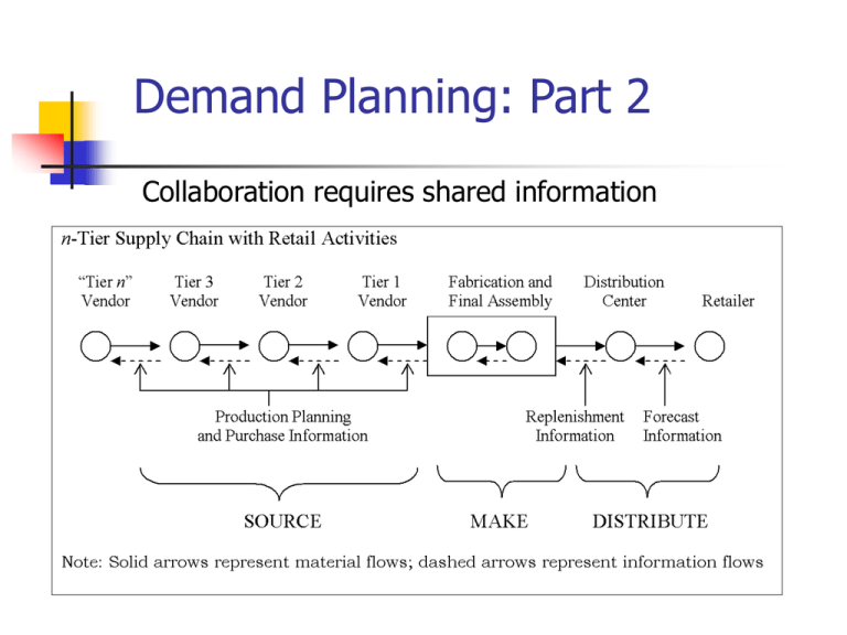
Demand Planning: Part 2
Collaboration requires shared information
1
Objectives





Hands on experience using smoothing
procedures
Enhanced trend and seasonal
smoothing models
Forecasting into the future
Parameter & initialization estimation
considerations
Error measures
2
Smoothing Models
Ft+1
Moving Average model
= Lt = (Dt + Dt-1 + ….+ Dt-n )/ n
Simple Exponential Smoothing
Ft+1 = Lt = α Dt + ( 1- α )Lt-1
Dt = sales in t
Lt = average in t
Ft = forecast in t
3
Forecasting Tools

Spreadsheets

Example: Excel





install the Data Analysis Toolpack (Tools/AddInns/Analysis Toolpack)
open the file containing the data
click on: Tools - Data Analysis (different options are
available)
Other Add-ins: e.g., KADD and StatTools
Forecasting application software (2 types)


statistical packages
forecasting packages specifically designed for
forecasting applications
4
Hands on Exercise

Hot Pizza exercise, problem 2, page 214


Use moving average (4 period) and simple
exponential smoothing (alpha = .2 & .4) models
with data, forecast weeks 13 to 16 into the future.
Northwestern Parts, (in class exercise for
seasonal and tend enhanced models)
5
Components of demand




Trend component: growth or decline
over an extended period of time
Cyclical component: wavelike
fluctuation around the trend
Seasonal component: pattern of change
that repeats itself year after year
Random component: after removal of
other components
6
Pattern Issues




Which patterns are present in data?
Things are not constant over time
Need a process to identify change
Need a procedure to update quickly
Enhancing Smoothing Procedures
7
Grow in Sales
Trend Pattern
700
600
Units
500
400
300
200
100
0
0
4
8
12
16
20
24
28
32
36
Quarter
8
Expo with Trend - Update Equations and
Forecasting Model
Basic Exponential Smoothing: Ft+1 = Lt = α Dt + ( 1- α )Lt-1
Update Equations with Trend:
Level:
Lt = α ( Dt ) + ( 1- α ) ( Lt- 1+Tt-1 )
Trend: Tt = β (Lt - Lt-1 ) + ( 1- β ) Tt-1
Forecast Equation for ‘n’ period in the future:
Dt = sales in t
Lt = average in t
Tt = trend in t
Ft = forecast in t
Ft+n = Lt + n Tt
9
Trend Adjustment


Update smoothed average for recent trend
Update Trend Factor


Difference of two period “Average”
Weighted combination of



Past trend factor
Current Forecast of trend factor
Trend the forecast
10
Seasonal Sale Pattern
Season Pattern
700
600
Units
500
400
300
200
100
0
0
4
8
12
16
20
24
28
32
36
Quarter
11
Expo with Season - Update Equations
and Forecasting Model
Basic Exponential Smoothing: Ft+1 = Lt = α Dt + ( 1- α )Lt-1
Update Equations:
Level:
Lt = α ( Dt / St ) + ( 1- α ) ( Lt- 1)
Season: St+p = γ ( Dt / Lt ) + ( 1- γ ) St
Forecast Equation for ‘n’ period in the future:
Ft+n = (Lt ) St+n
Dt = sales in t
Lt = average in t
St = season in t
Ft = forecast in t
p = season
12
Seasonality Adjustment



Deseasonalize recent sales data
Calculate smoothed average
Update Seasonal Factor


Ratio of Actual to “Average”
Weighted combination of



Past deseasonalized seasonal factor
Current Forecast of seasonal factor
Seasonalize the forecast
13
Trend & Seasonality Common
Coca Cola Quarterly Sales in Millions of Dollars
$5,500
$5,000
$4,500
$4,000
$3,500
$3,000
$2,500
$2,000
$1,500
196
Q
395
Q
195
Q
394
Q
194
Q
393
Q
193
Q
392
Q
192
Q
391
Q
191
Q
390
Q
190
Q
389
Q
189
Q
388
Q
188
Q
387
Q
187
Q
386
Q
Q
186
$1,000
14
Trend & Season (Winter’s) Update
Equations and Forecasting Model
Update Equations:
Level:
Lt = α ( Dt / St ) + ( 1- α ) ( Lt- 1+Tt-1 )
Trend: Tt = β (Lt - Lt-1 ) + ( 1- β ) Tt-1
Season: St+p = γ ( Dt / Lt ) + ( 1- γ ) St
Forecast Equation for ‘n’ period in the future:
Ft+n = (Lt + n Tt ) St+n
Dt = sales in t
Lt = average in t
Tt = trend in t
St = season in t
Ft = forecast in t
p = season
15
Forecast Error

Building a Forecast



Fit to historical data
Project future data
Forecast Error



How well does model fit historical data?
Do we need to tune or refine the model?
Can we offer confidence intervals about
our predictions?
16
Measuring Forecast Error

MAD or MAE


Bias (tendency measurement)


Sum of all errors (plus & minus)
MAPE (mean absolute percentage error)


average of the absolute errors
Average absolute ratio of error to actual
MSE (mean square error)

Square of all errors divided by ‘n’
17
Evaluating Forecast Models
with Different Measures




Error in period t
Mean Absolute
Deviation
Mean Absolute
Percentage Error
Mean Squared Error
et = d t - f t
n
MAD = S d t - f t
n
t =1
MAP =
E
n
n
S
t =1
(
dt - ft
n
dt
MSE = S d t - f t
t =1
(100 )
)
2
n
18
Mabert Web Page


Prepare: Specialty Packaging Corp. (A), pp.
216-217. Develop forecasts for each quarter
of 2007 for Clear and Black Plastic
containers. Seasonal time series. Try using
KADD analysis tool vs. provided Excel
workbook.
Quiz: There will be a short quiz covering the
fundamentals of demand planning and
smoothing forecast models. Open book and
notes.
19
Mabert Web Page

URL address with useful files:

http://kelley.iu.edu/mabert/class-e730.html
20