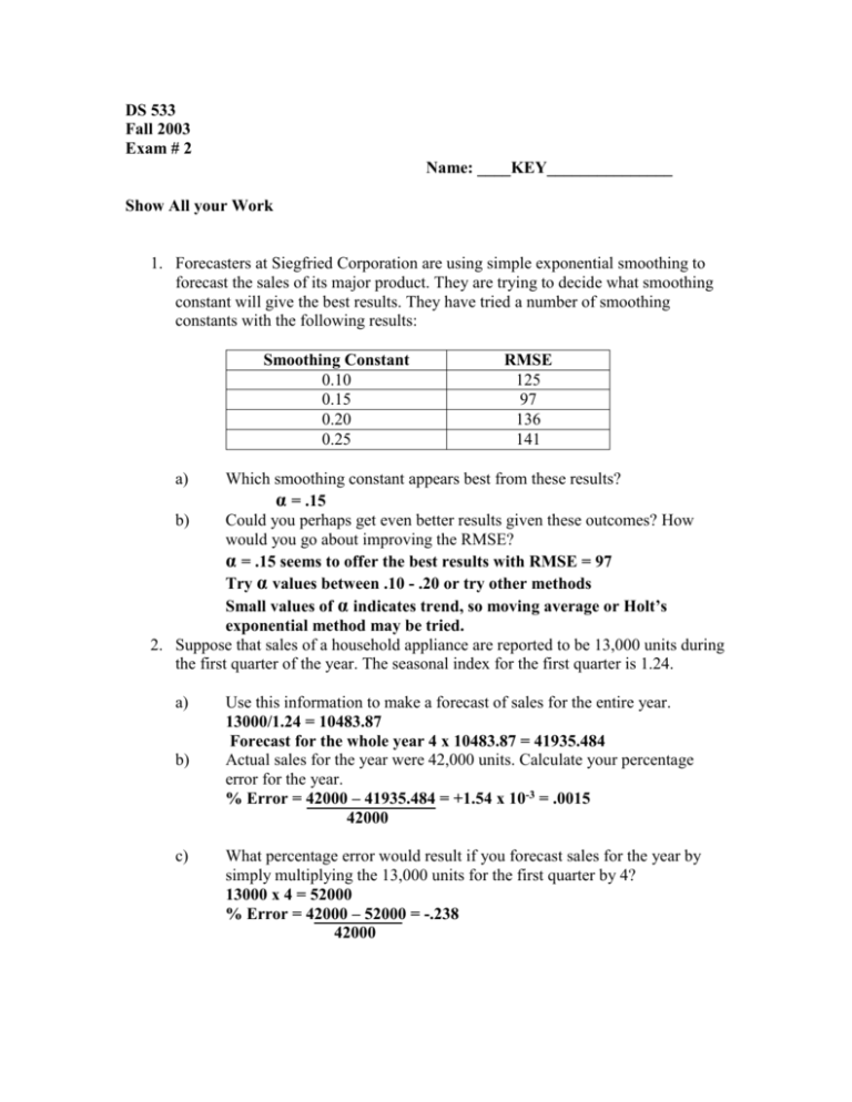
DS 533
Fall 2003
Exam # 2
Name: ____KEY_______________
Show All your Work
1. Forecasters at Siegfried Corporation are using simple exponential smoothing to
forecast the sales of its major product. They are trying to decide what smoothing
constant will give the best results. They have tried a number of smoothing
constants with the following results:
Smoothing Constant
0.10
0.15
0.20
0.25
RMSE
125
97
136
141
a)
Which smoothing constant appears best from these results?
α = .15
b)
Could you perhaps get even better results given these outcomes? How
would you go about improving the RMSE?
α = .15 seems to offer the best results with RMSE = 97
Try α values between .10 - .20 or try other methods
Small values of α indicates trend, so moving average or Holt’s
exponential method may be tried.
2. Suppose that sales of a household appliance are reported to be 13,000 units during
the first quarter of the year. The seasonal index for the first quarter is 1.24.
a)
b)
c)
Use this information to make a forecast of sales for the entire year.
13000/1.24 = 10483.87
Forecast for the whole year 4 x 10483.87 = 41935.484
Actual sales for the year were 42,000 units. Calculate your percentage
error for the year.
% Error = 42000 – 41935.484 = +1.54 x 10-3 = .0015
42000
What percentage error would result if you forecast sales for the year by
simply multiplying the 13,000 units for the first quarter by 4?
13000 x 4 = 52000
% Error = 42000 – 52000 = -.238
42000
3. The data in the table below give quarterly sales of the popular game Oligopoly at
the J-Mart variety store.
Year
1
Quarter
1
2
3
4
1
2
3
4
1
2
3
4
2
3
Time
1
2
3
4
5
6
7
8
9
10
11
12
a)
Find a four period moving average for each quarter.
b)
Find the centered moving averages for the sample.
c)
Find the seasonal factors. Report your results in the following table
Year
Quarter
Time
Oligopoly Sales
1
1
2
3
4
1
2
3
4
1
2
3
4
1
2
3
4
5
6
7
8
9
10
11
12
20
25
35
44
28
29
43
48
24
37
39
56
2
3
Oligopoly Sales
20
25
35
44
28
29
43
48
24
37
39
56
MA
CMA
SF
31
33
34
36
37.25
36
38
37
39
32
33.5
35
36.625
36.625
37
37.5
38
1.09
1.31
.8
.79
1.17
1.29
.64
.97
d)
Consider using the multiplicative decomposition method to forecast Oligopoly
sales for year 4 given the following information:
a. The centered moving average trend (CMAT) is estimated as
CMAT=24.1+1.8(time)
b. The seasonal index (SI) and cyclic factor (CF) are given below:
Year
Quarter
Time
Oligopoly Sales
1
1
2
3
4
1
2
3
4
1
2
3
4
1
2
3
4
1
2
3
4
5
6
7
8
9
10
11
12
13
14
15
16
20
25
35
44
28
29
43
48
24
37
39
56
2
3
4
e)
CMAT
SI
CF
47.5
49.3
51.1
52.9
0.71
0.87
1.12
1.29
0.71
0.87
1.12
1.29
0.71
0.87
1.12
1.29
0.71
0.87
1.12
1.29
1.08
1.07
1.06
1.05
0.99
0.96
0.93
0.90
1.01
1.00
0.98
0.93
0.90
1.00
Given the actual values shown in the following table, calculate the root mean
squared error (RMSE) for the year 4.
Period
Year 4 Q1
Year 4 Q2
Year 4 Q3
Year 4 Q4
Oligopoly sales
Actual
Forecast
30
33.0505
36
39.8886
39
51.5088
65
68.241
Sum of Squared Errors = 191.4010
Mean squared Error = 47.85
Root Mean Squared Error = 6.917
Squared Error
9.3056
15.1212
156.4701
10.5041
4.
Public sector economists routinely require unemployment forecasts in budget planning
and revenue projections. Consider the following time-series plot of the U.S.
unemployment rate over the period 1980M1-1997M4:
Given the graph above, which smoothing model(s) may be the most appropriate? What factors
may explain this?
As the data shows appreciable trend and no pronounced seasonality, candidate
models are moving averages, simple exponential smoothing.
Multiple Choice Questions
Select the best Answer
1.
Which method uses an arithmetic mean to forecast the next period?
A)
B)
C)
D)
2.
Which method is used to develop a simple model that assumes that weighted averages of
recent periods are the best predictors of the future?
A)
B)
C)
D)
E)
3.
Naive.
Moving averages.
Exponential smoothing.
None of the above
Naive.
Moving averages.
Exponential smoothing.
Naïve model squared.
None of the above
Simple-exponential smoothing models are useful for data, which have
A)
B)
C)
D)
E)
a downward trend.
an upward trend.
neither an upward or downward trend.
pronounced seasonality.
All the above.
Note: The next three questions relate to the following data:
Actual Series
100
110
115
Time Period
1
2
3
4.
Forecast Series
100
---
Forecast Error
0
---
If a smoothing constant of .3 is used, what is the exponentially smoothed forecast for
period 4?
A)
B)
C)
D)
E)
106.6.
103.0.
115.0.
112.6.
104.4.
5.
What is the forecast error for period 3?
A)
B)
C)
D)
E)
6.
If a three-month moving-average model is used, what is the forecast for period 4?
A)
B)
C)
D)
E)
7.
-3.
-12.
-10.
-7.
+7.
104.4.
106.6.
107.1.
108.3.
110.2.
Holt's smoothing is best applied to data that are
A)
B)
C)
D)
E)
nonseasonal.
nonstationary.
deseasonalized with a trend.
nonstationary and nonseasonal.
All the above.
8.
How many first initial values must the forecaster set using Winter's exponential
smoothing?
A)
B)
C)
D)
E)
9.
0.
1.
2.
3.
None of the above.
Which of the following is not a component in the time series decomposition model?
A)
B)
C)
D)
E)
Trend.
Seasonal variation.
Irregular variation.
Business indicators.
Cyclical variation.
10.
11.
When calculating centered moving-averages using a 4-period moving average, how many
data points are lost at the beginning of the original series?
A)
1.
B)
2.
C)
3.
D)
4.
E)
None of the above.
A seasonal index number of .80 for quarter one of an automobile parts manufacturer
suggests
A)
B)
C)
D)
E)
12.
Quarter one sales are 80% above the yearly norm.
Quarter one sales are 1.80% below the yearly norm.
Quarter one sales are 20% below the yearly norm.
Quarter one sales are 80% below the yearly norm.
None of the above.
The sum of seasonal index numbers for monthly data should equal
A)
B)
C)
D)
E)
one.
sample size/2.
4.
12.
None of the above.
Formulas
Moving average
Exponential Smoothing
( yt  yt 1  yt  2    yt  k 1 )
K
Holt’s method
yˆt 1   yt  (1   ) yˆ t
yˆ t 1 
yˆ t 1  yˆ t   ( yt  yˆ t )
Tt   ( Lt  Lt 1 )  (1   )Tt 1
Lt   yt  (1   )( Lt 1  Tt 1 )
yˆ t  p  Lt  pTt
Winter’s method
Lt  
yt
 (1   )( Lt 1  Tt 1 )
St  p
St  
Tt   ( Lt  Lt 1 )  (1   )Tt 1
yt
 (1   ) St  p
Lt
yˆ t m  ( Lt  mTt ) St  m p
Decomposition method
Yt  Tt  Ct  St  I t
SFt 
Yt
CMAt
Yt  Tt  Ct  St  I t
CF 
CMA
CMAT
CMAT  a  b(Time)
Errors
MAE 
1 n
 yt  yˆ t
n t 1
MSE 
1 n
( yt  yˆ t ) 2

n t 1
MAPE 
MPE 
n
RMSE 
(y
t 1
t
 yˆ t ) 2
n
1 n y t  yˆ t
 y
n t 1
t
1 n ( yt  yˆ t )
 y
n t 1
t