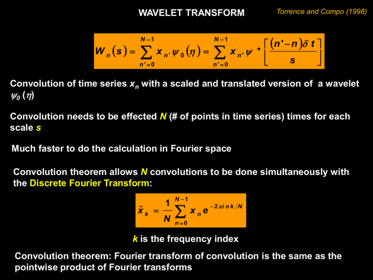
WAVELET TRANSFORM
Torrence and Compo (1998)
  n'  n  t 
W n s  
x n '  0   
x n'  * 

s


n'  0
n'  0
N 1
N 1


Convolution of time series xn with a scaled and translated version of a wavelet
0 ()
Convolution needs to be effected N (# of points in time series) times for each
scale s
Much faster to do the calculation in Fourier space
Convolution theorem allows N convolutions to be done simultaneously with
the Discrete Fourier Transform:
xˆ k 
1
N
N 1

xne
 2i n k N
n0
k is the frequency index
Convolution theorem: Fourier transform of convolution is the same as the
pointwise product of Fourier transforms
WAVELET TRANSFORM
  n'  n  t 
W n s  
x n'  * 

s


n'  0
N 1

xˆ k 
1
N
N 1
x
n
e
 2i n k N
n0
 t 
ˆ  s    Fourier transform of   
s
Inverse Fourier transform of Wˆ  xˆ kˆ
W n s  
N 1

is Wn (s)
i n  t
xˆ k ˆ *  s  k  e k
k 0
With this relationship and a FFT routine, can calculate
the continuous wavelet transform (for each s) at all n
simultaneously
k
N
 2 k
 N  t : k  2
 
2 k
N

: k 
 N  t
2
N 1
W n s  
 xˆ
k
ˆ *  s  k  e

k 0
1 4

i k n  t
e
i  0

e
2

2
1 4
H  e
 s  s 0
2
2
ˆ 0
0
To ensure direct comparison from one s to the
other, need to normalize wavelet function
 2 s 

ˆ  s  k   

 t 
12
2
ˆ 0  s  k

m
m
i m!
 2 m !

1 
i 
2
  m  1
m
H   s   e
m
m  2 m  1!
 s
ˆ 0
0


ˆ 0  '  d  '  1
2
  1

i.e. each unscaled wavelet function has
been normalized to have unit energy

0

0
m 1
d
m
1  d

 m  
2

m
e

2
2

ˆ 0
and at each scale (N is total # of points):
N 1

ˆ  s  k

2
 N
k 0
Wavelet transform is weighted by amplitude of
Fourier coefficients xˆ k and not by ˆ
ˆ 0
i

m
 m 

1

2
 s  m e   s  
2
2
W n s  
N 1

i n  t
xˆ k ˆ *  s  k  e k
k 0
Wavelet transform Wn(s) is complex because wavelet function  is complex
Wn(s) has real and imaginary parts that give the amplitude and phase
and the wavelet power spectrum is |Wn(s)|2
for real  the imaginary part is zero and there is no phase
 W n s 
for white noise
2

2
2
 N   xˆ k
  W n s 
2
Normalized wavelet power spectrum is W n  s 
2
 xˆ k

N
2


2
2
for all n and s
Seasonal SST averaged over Central Pacific
W n s 
2

2
Power relative
to white noise
Considerations for choice of wavelet function:
1) Orthogonal or non-orthogonal:
Non-orthogonal (like those shown here)
are useful for time series analysis.
Orthogonal wavelets – Haar, Daubechies
2) Complex or real:
Complex returns information on
amplitude and phase; better adapted for
oscillatory behavior.
Real returns single component; isolates
peaks
3) Width (e-folding time of 0):
Narrow function -- good time resolution
Broad function – good frequency resolution
4) Shape:
For time series with jumps or steps – use
boxcar-like function (Haar)
For smoothly varying time series – use a
damped cosine (qualitatively similar
results of wavelet power spectra).
2s

ˆ 0
0
s

2
ˆ 0
0
2s

ˆ 0
0
2s

ˆ 0
0
Cone of Influence
2s
Morlet & DOG
s
2
Paul
Seasonal SST averaged over Central Pacific
W n s 
2

2
Relationship between Wavelet Scale and Fourier period
Write scales as fractional powers of 2:
J 
log
2
N  t
j j
,
j  0 ,1,  , J
s0 
 j
smallest resolvable scale
should be chosen so that the equivalent
Fourier period is ~2  t
largest scale
W n s 
s j  s0 2
 j ≤ 0.5 for Morlet wavelet; ≤ 1 for others
2

2
N = 506
 t = 0.25 yr
s0 = 2 t = 0.5 yr
 j = 0.125
J = 56
57 scales ranging from 0.5 to 64 yr
Relationship between Wavelet Scale and
Fourier period 
 

0
Can be derived substituting a cosine wave of
a known frequency into
W n s  
N 1
 xˆ
k
ˆ *  s  k  e
4 s
0 
2  0
2
ˆ 0
  1 . 03 s :  0  6
i k n  t
k 0
 

ˆ 0
0
and computing s at which Wn is maximum
0
2m  1
  1 . 396 s : m  4
 

4 s
ˆ 0
2 s
m 12
  3 . 974 s : m  2
  2 . 465 s : m  6

ˆ 0
0
Seasonal SST averaged over Central Pacific
How to determine
the significance
level?
  1 . 03 s :  0  6
W n s 
2

2
  3 . 974 s : m  2
Because the square of a
normally distributed real
variable is 2 distributed
with 1 DOF
 xk
 W n s 
2
2
is  2
2
should
be  2
2
At each point of the
wavelet power spectrum,
there is a 22 distribution
For a real function
(Mexican hat) there is a
12 distribution
Distribution for the local wavelet power spectrum:
W n s 

2
2

1
2
Pk  2
2
Pk is the mean spectrum at Fourier frequency k,
corresponding to wavelet scale s
SUMMARY OF WAVELET POWER SPECTRUM PROCEDURES
1) Find Fourier transform of time series (may need to pad it with zeros)
2) Choose wavelet function and a set of scales
 2 s 

ˆ  s  k   


t


3) For each scale, build the normalized wavelet function
4) Find wavelet transform at each scale
W n s  
N 1
 xˆ
k
ˆ *  s  k  e
12
i k n  t
k 0
5) Determine cone of influence and Fourier wavelength at each scale
6) Contour plot wavelet power spectrum
7) Compute and draw 95% significance level contour
ˆ 0  s  k
