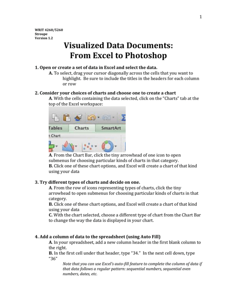
1
WRIT 4260/5260
Stroupe
Version 1.2
Visualized Data Documents:
From Excel to Photoshop
1. Open or create a set of data in Excel and select the data.
A. To select, drag your cursor diagonally across the cells that you want to
highlight. Be sure to include the titles in the headers for each column
or row
2. Consider your choices of charts and choose one to create a chart
A. With the cells containing the data selected, click on the “Charts” tab at the
top of the Excel workspace:
A. From the Chart Bar, click the tiny arrowhead of one icon to open
submenus for choosing particular kinds of charts in that category.
B. Click one of these chart options, and Excel will create a chart of that kind
using your data
3. Try different types of charts and decide on one.
A. From the row of icons representing types of charts, click the tiny
arrowhead to open submenus for choosing particular kinds of charts in that
category.
B. Click one of these chart options, and Excel will create a chart of that kind
using your data
C. With the chart selected, choose a different type of chart from the Chart Bar
to change the way the data is displayed in your chart.
4. Add a column of data to the spreadsheet (using Auto Fill)
A. In your spreadsheet, add a new column header in the first blank column to
the right.
B. In the first cell under that header, type “34.” In the next cell down, type
“36”
Note that you can use Excel’s auto-fill feature to complete the column of data if
that data follows a regular pattern: sequential numbers, sequential even
numbers, dates, etc.
2
C. Select the two cells in the column by dragging your cursor
D. Click and hold your cursor on the tiny blue square (handle) in the bottomright corner of the selected cells:
E. Without releasing the click, drag your cursor down the column to fill in
your data. Release when you get to where your column of data should end.
5. Update the chart to include the new column of data
A. On the chart, move your cursor over the portion of the chart where the
data is visualized until the tiny, yellow pop-up identifier reads “Plot Area.”
B. In that “Plot Area,” click once.
C. Over on the spreadsheet, you should see the columns and rows currently
displayed on the chart selected in light blue.
D. Move your cursor over the tiny blue handle in the bottom-right corner of
this selection until you see the cursor outline the handle with a box.
When you do, drag the handle to include the new column of data you just
added.
E. Your chart should now show the new data.
6. Resize the chart
A. Move your cursor to the bottom-right corner of your chart until your
cursor becomes a double-headed arrow, and then grab the three-dot “grip.”
B. Drag this grip toward the bottom right of the screen to enlarge the chart as
desired.
Generally speaking, it’s better to have a chart that’s too large rather than too
small. Once your convert this chart to an image, you can also reduce the size of
the image later without losing visual quality, but a chart that’s small can’t be
enlarged very much without showing ragged pixilation and rough edges.
7. Change the color of a chart element (or other format-able feature)
A. In the chart, click on one of the lines, bars, or pie slices. You should see
that element (and perhaps related chart elements) become selected with
handles on the corners.
B. Right-click on the selected element, and choose “Format Data Series”
C. From the “Format Data Series” window, make a selection for what you
want to change. For example, to reformat a line, choose “Line,” to reformat
part of a bar, choose “Fill.” You may need to experiment depending on the
kind of chart element you’re working with.
D. From the “Format Data Series” window next to “Color,” click the button
3
“Automatic” and choose a new color.
E. Click “OK” in the bottom corner of the “Format Data Series” window.
8. Save the Excel file
A. Click File > Save (or use the keyboard command “Command+s”
9. Save the chart as an image and then open it in Photoshop
A. In the chart, move your cursor to an empty corner of the chart until the
tiny, yellow pop-up identifier reads “Chart Area”
B. Right-click in this area, and from the pop-up menu choose “Save Picture
As…”
C. Save the chart as an image with a title you’ll recognize later.
D. In Photoshop, choose File > Open and navigate to the image file you just
saved to open it.
10. In a new Photoshop file, create a large image to use as a canvas for a
project. Save it as “october 9 sample” (but using today’s date). In these
directions, we’ll call this file “today’s sample.”
A. Open Photoshop, and choose File > New
B. In the “New” window, enter values for “Width” and “Height” appropriate
for a large image project intended for a screen (that is, landscape
orientation). Try 6000 Width and 1000 Height.
C. Adjust the size by choosing Image > Image Size. In the “Image Size”
window, unclick the “Constrain Proportions” box if necessary. Enter
new values for either Width or Height.
11. Copy the chart from its Photoshop document to the “today’s sample” file so
that the chart appears on its own layer. Resize and locate as desired.
A. Back in the chart image file, choose Select > All (or use the keyboard
short-cut “Command+a”)
B. Copy the selection by choosing Edit > Copy (or on the keyboard, hit
“Command+c”
C. Switch to the “today’s sample” file (select its tab at the top of Photoshop’s
document space), and paste the chart into the “today’s sample”
document (choose Edit > Paste, or use the keyboard shortcut
“Command+v”)
D. Look in the Layers Palette to see that Photoshop has created a new layer
for what you just pasted in. (If not, undo and create a new layer first.)
E. Resize the chart by choosing Edit > Transform > Scale. Photoshop will
place a bounding box around the pixels on the current layer (your
chart). Holding down the Shift key to maintain proportions, grab a
corner of the bounding box and drag outward to enlarge the chart,
inwards to shrink it.
F. Move the chart around in the document by choosing the Move Tool from
the Tool Palette (see below), and using the cursor to drag the chart to
where you want it to go.
4
12. Create a light-colored background in the “today’s sample” project (if
desired; or you can also use a large image as a background on its own layer)
A. In the “today’s sample” document, go to the bottom of the Layers Palette
and click the “Fill Layer” icon
B. From the menu, choose “Gradient”
C. From the “Gradient Editor” window, click the yellow/orange icon (or
another you prefer)
D. Under “Gradient Type” experiment with moving the sliders to adjust the
gradient in the document
E. Double-click the tiny color boxes on the sliders to open the “Color Picker”
and select new colors for various parts of the gradient.
F. Click OK in the “Gradient Editor”
G. In the Layers Palette, drag the new, gradient layer you just created to a
position under the chart’s layer in the palette’s stack of layers.
13. In the “today’s sample “document, eliminate the white background from the
chart so the background color shows through
A. In the Layers Palette, make sure you have the layer with the chart on it
selected (that it’s highlighted in blue). If not, click this layer in the
Layers Palette.
B. From the Tools Palette, select the Magic Wand Tool, which may be nested
under the Quick Selection Tool. The Quick Selection and Magic Wand
icons looks like this and this:
C. In the Properties Palette at the top (now showing the properties of the
Magic Wand Tool), make sure the checkbox next to “Contiguous” is not
checked
D. In the document, click once on the white background of the chart to
highlight it. All the white pixels on that layer should appear selected
(with the marching-ants circulating around it).
E. Hit “Delete”
Note: If Photoshop appears to have done a poor job in selecting all the
color you’ve tried to choose, you might try repeating this step with a
lower number in the Properties Palette’s box for “Tolerance.” Lower
tolerance means that Photoshop will be less tolerance of different colors:
that is, will select more colors similar to that of the pixel you clicked on
5
with the Magic Wand Tool.
14. Take a screen shot of a table of data from Excel, Word, or other software on
your computer to add to your “today’s sample” document in Photoshop.
A. In Excel, go to your original spreadsheet or other document. The following
steps, however, work with virtually anything you can see on your
computer screen.
B. Since you’re going to take a snapshot of how this file looks on your screen, make any
changes to the formatting, sizing, etc. so the content looks exactly as you
intend for it to appear in your project.
C. On a Mac, hit “command+control+shift+4” at the same time
D. Drag your cursor (which looks like crosshairs in a scope) diagonally to
select the area on your screen you want to copy to your computer’s
clipboard
E. In your “today’s sample” document in Photoshop, look at the bottom of the
Layers Palette for the “New Layer” icon and click it:
F. With the new layer selected in the Layers Palette, move you cursor
anywhere in the document and paste (choose Edit > Paste, or hit
“command+v”).
15. Clean up the extra pixels around the outside of the table (left over from
taking the screen shot) by doing the following. Delete the background
color in the table if desired.
A. In the Layers Palette, be sure you have the chart’s layer selected.
B. From the Tools Palette, choose the Rectangular Marquee Tool, which looks
like this:
C. In the document, drag diagonally to select the pixels (along one edge of the
table) which you want to get rid of.
D. Once you have selected those pixels, hit the “Delete” key
E. Repeat this process for the other edges of the table.
F. If desired, use the same technique that you used above for the chart to
eliminate the white (or other colored) background for the table.
6
16. Before you create your web-ready image from this Photoshop document,
resize the “today’s sample” image to be large enough to display the
content, but not so large as to be excessively huge at full size.
A. In the document “today’s sample,” choose View > Actual Pixels
B. Decide if the image, viewed at this full size, is too large or too small.
For images that you are preparing for use on the web, the goal is to make the
content large enough to be clearly visible/legible and easily understood on a
screen without strain. It’s okay if the image is a little too large for a browser
window. (We can never know the size of audience’s window, the settings of her
monitor, or lots of other variables that affect the size of what the viewer will
actually see.) Web browsers will, by default, shrink a too-large image to fit in
the available screen space, giving the user the option to click once on the image
to make it display full size, and then click again to return it to its shrink-to-fit
size. Nevertheless, if the full sized version is ridiculously tall and/or wide, it
looks like a mistake. It also means that the image file takes longer to download
than necessary.
C. Choose Image > Image Size
D. Be sure the checkbox “Constrain Proportions” at the bottom of the “Image
Size” window is checked.
E. In the “Pixel Dimensions” area, use the drop down menus to the right of
“Width” and “Height” to choose “Pixels” as the unit of measure.
F. Enter values for “Width” and “Height”: try 1,600 pixels wide and 1,000
pixels high.
G. Click OK
H. See how the size suits you. Repeat as necessary.
17. Save the “today’s sample” file, and then save a version for the Web .
A. Hit “control+s” or choose File > Save
B. Choose File > Save for Web
C. From the “Save for Web” window, choose the “4 Up” Tab.
D. From the four panes, experiment with different settings and file formats using the
control panel on the upper right of the window.
E. With your cursor, select the panel with the best combination of visual quality and
small file size
F. Hit “Save” at the bottom