Proceedings of the Twenty-Ninth AAAI Conference on Artificial Intelligence
DynaDiffuse: A Dynamic Diffusion Model for
Continuous Time Constrained Influence Maximization
Miao Xie1,2,3 , Qiusong Yang2,3 , Qing Wang2,3 , Gao Cong4 , Gerard de Melo5
1
2
University of Chinese Academy of Sciences, China, {xiemiao, qiusong, wq} @nfs.iscas.ac.cn
National Engineering Research Center of Fundamental Software, Institute of Software, Chinese Academy of Sciences
3
State Key Laboratory of Computer Science, Institute of Software, Chinese Academy of Sciences, China.
4
School of Computer Engineering, Nanyang Technological University, Singapore, gaocong@ntu.edu.sg
5
Tsinghua University/Microsoft Research Asia, China, gdm@demelo.org
Abstract
In this paper, we thus drop the assumption of a static
network and investigate how to account for network evolution in influence maximization. We define the continuous time constrained influence maximization problem
and propose the continuous time dynamic diffusion model
(DYNA D IFFUSE) for dynamic diffusion networks. Having
captured specific dynamic characteristics of networks (such
as herd behavior and activeness), DYNA D IFFUSE enables
us to consider their effects while estimating the influence
spread of a set of nodes within a given time frame. This is
achieved using an innovative stochastic model checking approach. Although the new problem is NP-hard, the influence
spread function is monotonic and submodular. This enables
us to obtain fast approximations with a lower bound precision ratio of 1 − 1/e. In our experiments on real social network data, we show that network evolution indeed plays an
important role in influence maximization. DYNA D IFFUSE
leads to significantly more influential node sets than previous models, with negligible time overhead.
Studying the spread of phenomena in social networks is
critical but still not fully solved. Existing influence maximization models assume a static network, disregarding
its evolution over time. We introduce the continuous
time constrained influence maximization problem for
dynamic diffusion networks, based on a novel diffusion
model called DYNA D IFFUSE. Although the problem is
NP-hard, the influence spread functions are monotonic
and submodular, enabling fast approximations on top
of an innovative stochastic model checking approach.
Experiments on real social network data show that our
model finds higher quality solutions and our algorithm
outperforms state-of-art alternatives.
1
Introduction
Understanding how information, diseases, etc. spread in a
network is vital in many settings. Companies may wish to
target users such that they, by word-of-mouth, influence their
friends, friends-of-friends, and so on, to purchase a product. Finding a set of initial nodes that will eventually influence the largest number of nodes in a network is critical
for achieving a high success rate (Domingos and Richardson
2001). Solving such an influence maximization problem can
enable us to predict the success or failure of new innovations
in their early stages, or to shape the process accordingly.
While several influence diffusion models have been proposed, all of them assume the given network is static (Guille
et al. 2013). In reality, however, networks may evolve quite
notably during the diffusion process (Mislove et al. 2008;
Tang et al. 2010). Matsubara et al. (2012) found that the information diffusion process often goes on for days or even
months. During this time, the degree of influence between
two nodes can change quite substantially due to changing interests or social ties. Likewise, the network topology
may change, with new nodes appearing or disappearing, and
edges coming and going. Gomez-Rodriguez, Leskovec, and
Schölkopf (2013) show that information diffusion networks
inferred from cascade data often evolve dramatically as the
information cascades accumulate. Accounting for such dynamics and thus pursuing seed node sets of a higher quality
may lead to significant financial gains.
2
Related Work
Kempe, Kleinberg, and Tardos (2003) first formulated the
problem of influence maximization in a graph, in which influence propagation is captured using stochastic cascades,
as in their independent cascade (IC) model. Recently, temporal aspects have been gaining increasing attention. Chen,
Lu, and Zhang (2012) incorporated the time delay of influence diffusion into the IC model. Liu et al. (2012) defined
a discrete time constrained information maximization problem and improved the IC model by adding the time stamps
of every time period for each edge, but their algorithms do
not consider continuous time constraints. Gomez-Rodriguez
and Schölkopf (2012) proposed a continuous time constrained diffusion model, which can be inferred from a cascade database (Gomez-Rodriguez, Balduzzi, and Schölkopf
2011). However, unlike DYNA D IFFUSE, all aforementioned
models assume a static network with fixed propagation rates
or probabilities during the diffusion process.
Finding the best initial set of nodes requires combinatorial optimization, which is very costly. Many studies aimed
at speeding up Kempe’s greedy algorithm. Kimura and Saito
(2006) introduced a shortest-path based IC model and provided efficient algorithms for it. Leskovec et al. (2007)
proposed the Cost-Effective Lazy Forward (CELF) scheme
c 2015, Association for the Advancement of Artificial
Copyright Intelligence (www.aaai.org). All rights reserved.
346
with potential diffusion edges and edge-specific propagation
rates directly from diffusion cascade data using an optimization algorithm. Then we can construct a Continuous Time
Markov Chain (CTMC) when given an initial set.
for selecting new seeds to significantly reduce the number of influence spread evaluations. Chen, Wang, and Yang
(2009) proposed two algorithms: MixedGreedy and DegreeDiscount. Liu et al. (2014) developed a heuristic algorithm based on independent influence paths. Furthermore,
Tang, Xiao, and Shi (2014) presented a greedy algorithm
called TIM by generating many random graph sets under
parameters control. Cohen et al. (2014) developed an efficient sketch-based algorithm (SKIM) by pre-generating a
small sketch for nodes. However, these algorithms all assume static networks with fixed propagation probabilities.
3
Definition 2. Continuous Time Markov Chain (CTMC):
A (labeled) CTMC is a tuple (S, s0 , R, L), where S is a finite
set of states and s0 ∈ S is the initial state. R : S ×S → R≥0
is a transition rate matrix assigning rates to pairs of states
with r ∈ R used as rate parameters of the exponential distribution f (t) = re−rt ,t > 0. We allow self-loops. Finally, for
a fixed finite set P of action labels, L : R → 2P is a function
assigning such labels to every transition with r > 0.
Problem Definition and Overview
We can create a CTMC (S, s0 , R, L), denoted by M0 ,
to represent the behavior of an inferred diffusion network
G(V, E) as follows. Each state s ∈ S has |V | dimensions,
with values of 0 or 1 representing whether a node has been
influenced. We first create an initial state s0 for I, the initial
set. For example, in Figure 1a and b, s0 = (1, 0, 0) represents that for I = {A} only A is initially influenced. Next,
we iteratively create all other reachable states in S and their
corresponding transitions in R. Iterating over A’s outgoing
edges, we find that nodes B and C can be influenced, so
we need two new states in S, (1, 1, 0) for reaching B and
(1, 0, 1) for reaching C, along with two associated transitions for them. If these states are already in S, we just need to
add transitions. We iterate this process until there is nothing
left to add. For a transition
from state s1 to s2 , the transition
P
rate is calculated as ei ri , where ri is the propagation rate
of each edge that can influence the new node. For example,
A and B in state (1, 1, 0) can independently influence C, so
the transition rate is r2 + r3 . Finally, we get four reachable
states in S plus associated transitions in R, and L = ∅.
Next, we consider dynamic properties of social networks
(Lang and Wu 2011, for example). It is impossible to model
all possible dynamics exhibited by different social networks.
However, having discovered salient dynamic characteristics from real data, we can capture these using additional
CTMC models. We introduce local variables f1 , . . . , fm ,
which model dynamic factors for a dynamic characteristic.
These factors are used to model the degree of effects on the
diffusion network by a positive function Φ(f1 , . . . , fm ). In
the CTMCs for dynamic characteristics, transitions can be
divided into two types: Internal transitions define how these
dynamic factors evolve stochastically, while external transitions associated with action labels will be used for synchronization with the main CTMC M0 defined earlier. M0 ’s
action labels will be updated to match these labels.
For example, Figure 1c presents a dynamic characteristic called activeness (detailed in Section 4.3). There is only
one state and one local variable step. The internal transition,
[]dr : step++, represents that step increases with rate dr,
where dr is a constant. The external transition, [AL]ddstep ,
is labeled with an action label AL indicating low activeness.
After defining dynamic characteristics, we update the corresponding action labels for M0 . If node C has low activeness
in Figure 1a, we add the action label AL for all transitions
that can influence C. The result is shown in Figure 1d. We
next explain how to connect these CTMCs to model the evo-
In contrast to previous work, our problem definition more
closely reflects real networks by allowing diffusion rates and
probabilities for each edge to vary during the diffusion.
Definition 1. Continuous time constrained influence
maximization problem for dynamic diffusion networks:
Suppose we are given (1) a social network snapshot
G(V, E), (2) a set of dynamic characteristics reflecting how
it will evolve, (3) a time bound T , and (4) a positive integer
k < |V |. Our goal is to find an initial set I ⊂ V of k nodes,
maximizing the expected total number of nodes influenced
up to time T , as estimated by an influence function σT (I).
Our solution to this problem consists of three parts:
1. In Section 4, we propose a new continuous time constrained dynamic diffusion model, called DYNA D IFFUSE.
2. In Section 5.1, an influence spread analysis method for
DYNA D IFFUSE, relying on stochastic model checking, is
given to estimate the influence of an initial set of nodes.
3. In Section 5.2, we design a fast greedy algorithm called
FAST M ARGIN after proving the monotonicity and submodularity of the influence function for DYNA D IFFUSE.
4
Dynamic Diffusion Model
We now present a new dynamic diffusion model
(DYNA D IFFUSE) and then derive a specific instantiation based on real social network data.
4.1
Model Definition
In our diffusion model, each node is either influenced or not.
Initially only a small set of nodes in an initial set I are influenced (by an external action such as supplying free product
samples). Then, every node in I tries to influence its adjacent neighbors. If a node has successfully been influenced,
it tries to influence its own neighbors, and so on. We assume
that once a node has been influenced, this state persists until
the end. The process terminates when there are no remaining
uninfluenced nodes or when the given time T has elapsed.
Whether a node succeeds in influencing its neighbor is
modeled using propagation rates. Clearly, different edges
have different propagation rates (Kossinets, Kleinberg, and
Watts 2008), and these may also change over time. Following previous work, we use the exponential distribution to
model the propagation rate. For an edge from node i to node
j associated with a propagation rate r, the influence diffusion probability is 1 − e−rt , where t is the time span after node i is influenced. We can infer a diffusion network
347
[]dr:step++
(1,1,0)
B
[]r1
r2
r1
(1,0,0)
r3
A
(1,0,0)
(b) CTMC for G, initial set I={A}, (1,0,0) is initial state
[AL] ddstep
[]r1
(1,0,1)
(c) CTMC for Activeness (d) Correlate with (c) by adding action labels for (b)
[]dr:step++
[AL](r2+r3). ddstep
[]r1
(1,1,1)
[AL]r3
[]r1
(1,0,1)
(a) Diffusion Network G
1
(1,1,0,1)
[]dr:step++
[AL]r2+r3
[]r1
(1,1,1)
[]r3
C
(1,1,0)
[]r2+r3
[]dr:step++
[]dr:step++
(1,0,0,1)
[AL]r3. ddstep
(1,1,1,1)
[]r1
(1,0,1,1)
(e) Parallel Composition for (c) and (d)
Figure 1: DYNA D IFFUSE modeling example, where dd stands for decreaseDelta and dr for decreaseRate
lution of the inferred network.
4.2
Definition 3. CTMC Parallel Composition: For two labeled CTMCs M1 = (S1 , s01 , R1 , L1 ) and M2 = (S2 , s02 ,
R2 , L2 ), the parallel composition, M1 k M2 , is a CTMC
(S1 × S2 , (s01 , s02 ), Rc , L1 ∪ L2 ), where Rc is defined as:
Algorithm 1 presents the complete modeling process for a
DYNA D IFFUSE instantiation. First, we make use of a convex optimization algorithm (Gomez-Rodriguez, Balduzzi,
and Schölkopf 2011) to infer the diffusion network topology G = (V, E) with R̄ as a set of propagation rates for
every edge (Figure 1a). Given an initial set, we can construct its corresponding CTMC M0 = (S, I, R, L) where
L is empty, i.e., L(r) = ∅ for all r ∈ R. Then, we model
each dynamic characteristic by a dynamic module di ∈ D
as a CTMC (Figure 1c). To establish their correlation, we
add action labels L of M0 for corresponding external transitions in di (Figure 1b). Finally we synchronize them by
following Definition 3 (Figure 1e). We can then use stochastic model checking to predict the influence spread in a given
time (Section 5.1).
α
[ι]s1 −→1 s01
α
[ι]hs1 , s2 i −→ hs01 , s2 i
ι ∈ L1 \ L2 , α ∈ R1
α
[ι]s2 −→2 s02
α
[ι]hs1 , s2 i −→ hs1 , s02 i
α1
[ι]s1 −→1 s01
ι ∈ L2 \ L1 , α ∈ R2
α2
[ι]s2 −→2 s02
∧
α1 ·α2
[ι]hs1 , s2 i −→ hs01 , s02 i ι ∈ L1 ∩ L2 , α1 ∈ R1 , α2 ∈ R2
α
Here, [ι]s −→ s0 means that the CTMC evolves from state
s to s0 when α ∈ R is performed with action label ι ∈ L.
Modeling Process
Algorithm 1 Complete Modeling Process
We can see that transitions with different action labels
in different Mi may only occur independently. In contrast,
transitions with the same action labels in different
Q Mi must
occur together with a combined transition rate i αi . The
combined CTMC with the activeness dynamic characteristic is shown in Figure 1d. In this example, if step is changed
during the simulation, the transition rates of subsequent transitions will evolve as [AL]r3 · ddstep .
In this way, we can model most common dynamic characteristics. If a new connection appears, we can introduce
an edge with a minimal positive value at the beginning that
increases later. An edge (re-)emerges when its rate increases
from the minimal value, and conversely an edge disappears
if its rate decreases to that value. Nodes can be regarded as
removed when all of their edges have disappeared.
With this modeling approach, we get a labeled CTMC M0
for an inferred diffusion network and a series of CTMCs
D = {d1 ...dn } for dynamic characteristics. Finally, we define the DYNA D IFFUSE model as follows.
Input: C (Cascade Data), T (time constraint), I (initial set)
1: G(V, E, R̄) ← gls(C, T )
# optimization algorithm
2: Create CTMC M0 = (S, I, R, L) from G, A
3: D ← dynamic modules mined from real data
4: modify L of M0 to capture the correlation with D
5: return M0 k D as DynaDiffuse
4.3
Salient Dynamic Characteristics
While DYNA D IFFUSE can flexibly capture various kinds of
network evolution, we focus on two important characteristics of information spread in social networks.
Herd Behavior. It is a well-established phenomenon that
over time, with an increasing number of influenced people,
propagation rates increase. The strength of this effect, however, differs for different types of users. Several studies show
that information diffusion is affected by a person’s conformity, i.e., inclination to be influenced (Li, Bhowmick, and
Sun 2011; Tang, Wu, and Sun 2013; Raafat, Chater, and
Frith 2009). For each user v, we compute a conformity score
Definition 4. Continuous Time Dynamic diffusion Model
(DynaDiffuse): Given a CTMC M0 for a network G =
(V, E), a set A of propagation rates αu,v for each (u, v) ∈
E, an initial set of vertices I ⊆ V , and a set of dynamic
characteristics D = {d1 , . . . , dn }, where each di ∈ D is
a CTMC model whose transition rate matrix represents a
given positive function Φ(f1 , . . . , fm ) (with dynamic factors
fj and Φ ≥ 0), DYNA D IFFUSE M is a synchronous CTMC
model defined as M = M0 k D = M0 k d1 k · · · k dn .
|{(m, v, t) ∈ Pv | ∃(m, v 0 , t0 ) : pv,v0 ∧ ≥ t − t0 ≥ 0}|
|Pv |
where Pv is the set of user v’s posting history logs, pv,v0 ∈
P , representing the posting logs that user v posted to user
v 0 and is a maximal time difference for v’s reposting of
348
Fraction of total messages
v 0 ’s posting (one week in our dataset from Section 6). Individual conformity represents how strongly v’s posting behavior conforms to that of her friends. In our dataset, we
discover that nearly 30% of users have a conformity > 0.6.
We divided the users into three groups according to their
conformity values and randomly selected 100 users from
each group to calculate the distribution of the times a posting had been reposted before they forwarded it. Our analysis
revealed that users with high conformity either repost very
popular postings or brand new ones posted by their close
friends, often related to their personal offline life. Low conformity users, in contrast, do not seem to show any clear
pattern. Therefore, we model herd behavior at different intensities for different conformity levels. Given a conformity
vector for all nodes, we define a CTMC as follows.
0.2
0.15
0.1
0.05
0
12
11
10
>0
9
8
7
6
5
Time (months before 2013.11)
>0.2
>0.4
4
>0.5
3
2
1
>0.7
Figure 2: Fraction of interactions over time for one year .
the user has posted or reposted (during a one week period
in our experiments). For analysis purposes, we divided the
users into groups according to their activeness values and
randomly selected 10% of users in each group to calculate
the average interaction levels based on one year of historic
data. Figure 2 illustrates that highly active users display a
relatively more even distribution of posting messages over
time, compared to other groups. On the contrary, less active
users post less and less over time. The trends are different
for different groups. To capture this, we thus divide the user
base into two parts using a threshold on their activeness. For
active nodes (whose activeness is larger than the threshold),
we assume stable transition rates for all of their incoming
edges during the diffusion process. On the contrary, the incoming edges’ transition rates for inactive nodes (low level
activeness) will stochastically decrease over time, following
an exponential distribution with expectation decreaseRate.
Given a classification threshold γ, the function Φ of this dynamic module can be expressed as
module “herd behavior”
n : [0..|V |] init by |I|;
/* conformity ≥ 60% */
[CH] n > 0 → 1 + ψ(n) ∗ conformityhigh : (n0 = n + 1);
/* 60% > conformity ≥ 30% */
[CM ] n > 0 → 1+ψ(n)∗conformitymiddle : (n0 = n+1);
/* conformity < 30% */
[CL] n > 0 → 1 + ψ(n) ∗ conformitylow : (n0 = n + 1);
end module
The module definition syntax used here is based on the
Reactive Modules formalism (Alur and Henzinger 1999),
with local variables and transition commands that reflect
the operational behavior of the module, i.e., state transitions of the CTMC. Here, the local variable n (with range
from 0 to |V |) represents the current number of influenced
nodes, which is initialized as |I|. The form of each transition command is [action label] guard condition → rate :
updates. Updates can be performed if and only if the current state of the CTMC meets the guard condition. We label each node’s incoming edge by its conformity level in
the CTMC for the inferred diffusion network, with [CH]
for high, [CM ] for medium, and [CL] for low conformity.
For each level i, conformityi is the average value for all
nodes at this level. The transition rate function Φ(n) =
1 + ψ(n) · conformityi models the changing trend of the
rate as the number of influenced
−1 users increases. We define
n
−δ ( |V
−b)
|
ψ(n) = γ 1 + e
for γ > 0, as this mirrors
the spread process for popular events in a network, first increasing gradually at an increasing rate and then stabilizing.
The range of ψ(n) is determined by γ, the curve’s slope by δ,
and b is the rate’s breakpoint. In our experiments, we study
how these variables affect the initial set selection for influence maximization.
step


decreaseDelta
Φ =


1

activeness < γ
otherwise
Then, given an activeness vector of all nodes, we define
the activeness module using a label AL for low activeness
and a parameter decreaseRate to control the evolution.
module “Activeness”
const float decreaseRate;
const float decreaseDelta;
step : [0..IntMax] init by 0;
[] step ≥ 0 → decreaseRate : (step0 = step + 1);
[AL] step > 0 → decreaseDeltastep : (step0 = step);
end module
5
Influence Analysis and Maximization
We now define the influence function for the DYNA D IFFUSE
model and apply our novel stochastic model checking approach to predict the influence spread.
Activeness of Actors. Studies (Lang and Wu 2011;
Viswanath et al. 2009) show that social actors exhibit different levels of activeness. In particular, highly active ones
contribute more towards the interaction, e.g. by reposting
messages and posting new stories. Although there are many
other factors, such as user interests, beliefs, and topics, much
of their effects can be attributed to a user’s activeness.
From our real diffusion dataset (cf. Section 6), we
first measure the activeness of every node v ∈ V as
activeness(v) = |vp |, i.e., the total number of messages
5.1
Spread Analysis
Definition 5. The influence spread σT (I) of an initial set I
until time T in a DYNA D IFFUSE model MI is defined as the
expected number of nodes influenced until T :
σT (I) = ENT (I) =
|V |
X
P (ti ≤ T |MI ),
i=1
where ti denotes the time when node i is influenced.
349
To estimate the influence spread of a given initial set I, we
rely on stochastic model checking (Kwiatkowska, Norman,
and Parker 2007), a method for computing possible behaviors of a stochastic system. Given a model description and
a formula in temporal logic, stochastic model checking provides the likelihood of the model satisfying the formula as
well as a wider range of quantitative measures relating to
model behavior. For example, one can use stochastic model
checking to determine the expected running time or expected
number of lost messages of a system.
Transitions (except self-loops) of the DYNA D IFFUSE
model correspond to non-influenced nodes becoming influenced. To calculate ENT (I), we tie a reward to every such
transition, and accumulate all rewards in the diffusion process to estimate the number of influenced nodes. Given a
DYNA D IFFUSE model M , we denote the instantaneous reward associated with the transition from state i to state j as
rewardij . The reward Markov process associated with M is
then (M, REM ), where the reward accumulated in the time
Rt
interval (0, t] is REM = 0 rewardM (u−),M (u) dNM (t),
where NM (t) is the number of state transitions of M in the
time interval (0, t]. Assume rewardij = 1 for all transitions.
Rt
P|V |
Then REM = 0 dNM (t) =
i=1 P (ti ≤ T |MI ). This
can be determined using a Uniformisation based Stochastic Model Checking approach (Kwiatkowska, Norman, and
Parker 2007). It allows us to either get an exact result by
verification, or to estimate the result using a faster simulation approach. In our study, we used the PRISM system
(Kwiatkowska, Norman, and Parker 2011) for this.
5.2
Theorem 3. The influence function σT (I) for DYNA D IFFUSE is submodular.
Proof. Consider any set of nodes V1 ⊆ V2 ⊆ V , and a node
v0 ∈ V \ V2 (if V2 = V , then trivially V01,T = V02,T below). We again use ∆x ∈ χ, as in the proof of Theorem 2.
We assume ∆V0i,T is the set of nodes that can be reached
from v0 , but cannot be reached by Vi (i = 1, 2) within the T
bound in the ∆x graph. Since V1 ⊆ V2 , we obtain ∆V01,T ≥
∆V02,T . We see that σT,∆x (V1 ∪ {v0 }) − σT,∆x (V1 ) =
∆V01,T ≥ ∆V02,T = σT,∆x (V2 ∪ {v0 }) − σT,∆x (V2 ) and
thus σT,∆x (I) is submodular. From this it follows that σT (I)
is submodular, concluding the proof.
FAST M ARGIN Greedy Algorithm. The standard greedy
algorithm for maximizing monotonic and submodular functions has a provable lower bound ratio of 1 − 1/e. However, for genuine scalability, we propose a faster marginal
influence spread estimation algorithm for the continuous
time diffusion model. Our algorithm (Algorithm 2) first predicts a relatively precise influence spread using stochastic model checking on the CTMC Parallel Composition.
Then, we predict the increased marginal influence spread
(σT (I ∪{v})−σT (I)) of adding each v ∈ V \I when selecting an additional node to be added to the current initial set.
To improve the efficiency, we estimate this marginal influence spread using a faster discounted formula for σT ({v}) in
Line 12, instead of determining a precise value with stochastic model checking.
Algorithm 2 FAST M ARGIN Greedy algorithm
Scalable Influence Maximization
Require: a DYNA D IFFUSE for a graph G = (V, E), the size k of
the desired initial set, a time constraint T
1: I ← ∅;
2: for each v ∈ V do
3:
predict accurate σT ({v}) using stochastic model checking
4: u ← argmaxv (σT ({v}))
5: I ← {u}
6: for i ← 2 to k do
7:
for each v ∈ V \ I do
8:
if (v, u) ∈ E and u ∈ N (I) then
9:
PI,u ← 1 − Π(w,u)∈E,w∈I (1 − e−ru,w (T ) )
10:
else
11:
PI,u ← 0
12:
∆σT ({v}) ← σT (I ∪ {v}) − σT (I)
Complexity, Monotonicity, and Submodularity.
Theorem 1. Continuous time constrained influence maximization on a DYNA D IFFUSE model is NP-hard.
Proof. With dynamic modules D = ∅ and T → ∞, our
DYNA D IFFUSE model turns out to be an instance of the independent cascade model. Hence, the latter is a special case
of DYNA D IFFUSE. As the traditional influence maximization problem is known to be NP-hard (Kempe, Kleinberg,
and Tardos 2003), this new problem is also NP-hard.
Theorem 2. The influence function σT (I) for DYNA D IFFUSE is monotonous.
≈ σT ({v})
Proof. If initial nodes are influenced at t = 0, each transition (except self-loops) of a DYNA D IFFUSE model means
there will be a new influenced node. The time delay is determined by an exponential distribution with a step-varied
expectation value. Consider the possible distributions of all
possible time differences between each pair of states in the
model. There will be a series of different state graphs χ. For
a given ∆x ∈ χ, we define σT,∆x (I) as equal to the number
of nodes reachable from I by at least one path with length no
larger than T . It is very natural to discover that σT,∆x (S) ≤
σT,∆x (S ∪ v) (for S ⊂P V ). Therefore, σT,∆x (I) is
monotonous. As σT (I) = ( x∈χ σT,∆x (I))/|χ|, we obtain
that σT (I) is monotonous as well.
Σ(v,u)∈E (1−e−rv,u (T ) )(1−PI,u )σT ({u})
Σ(v,u)∈E (1−e−rv,u (T ) )σT ({u})
13:
u ← argmaxv (∆σT ({v}))
14:
I ← I ∪ {u}
15: return I
# using CELF
# best set I
Here, N (I) is the set of directed successors of I, and PI,u
is the probability that u is influenced immediately by current
initial nodes. We estimate the probability with an exponential distribution for the whole diffusion period. The discount
is to subtract the influence spread that may be obtained by
I from σT ({v}). The higher the probability that v’s neighbors are already influenced by I, the larger the discount that
should be applied to σT ({v}). For scalability to large networks, we also adopt the CELF lazy evaluation approach
350
(Leskovec et al. 2007), which dramatically reduces the number of evaluations of argmaxv (σT (I ∪ {v}) − σT (I)). We
call this algorithm FAST M ARGIN. This algorithm can flexibly be used in any continuous-time constrained diffusion
model that assumes that the diffusion rate follows the exponential distribution.
Time and space complexities. Let dmax be the maximum degree of all nodes, and S and R be the states and
transition matrix of a DYNA D IFFUSE instance, respectively.
In Algorithm 2, the first for loop requires O(|V ||S|2 ) time
for uniformisation. The second for loop will cost O((k −
1)|V |dmax ). So the total runtime complexity is O(|V ||S|2 +
(k − 1)|V |dmax ). However, the standard greedy algorithm’s
time complexity is O(k|V ||S|2 ). Thus, they have the same
running time when k = 1, and Algorithm 2 is faster for
k > 1. The space complexity is O(|V |(|S| + |R|)), dominated by stochastic model checking in line 3.
1200
800
(a)
600
800
Influence spread
Influence spread
(b)
700
1000
600
400
200
500
400
300
200
100
0
0
2
4
6
8
10
12
14
16
0
18
0
1
2
3
4
5
6
7
Time horizon
FastMargin-Dynamic(Slow)
FastMargin-Dynamic(Quick)
FastMargin-Static
Real
K, size of initial set
FastMargin-Dynamic
FastMargin-Static
CELF-Dynamic
CELF-Static
CELF-IC
Figure 3: (a) Diffusion models comparison by DYNA D IFFUSE
with T = 3 days. Herd behavior module: δ = 30, b = 0.05, activeness module: decreaseDelta = 0.9, decreaseRate = 0.2. (b)
Comparison by the real influence spread with K = 6. Slow evolution: δ = 30, b = 0.05, decreaseDelta = 0.9, decreaseRate =
0.2. Quick evolution: δ = 100, b = 0.01, decreaseDelta = 0.9,
decreaseRate = 0.4. Legend: greedy algorithm–diffusion model
Computing Time(s)
140000
6
Experimental Evaluation
Dataset. We evaluate our model and algorithm on a microblog diffusion dataset from Sina Weibo, a major Chinese
microblogging platform. The data covers 96, 700 users and
373, 412 microblog postings (211, 052 original and 162, 360
reposted) from the time period of November 2–8, 2013. For
each of these postings, it contains a set of time-stamped
reposting logs with user ID, reposting time, and reposting
contents, in total nearly 4, 000, 000 entries. From this data,
we inferred an underlying diffusion network with 6, 000
top nodes and the 30, 000 fastest edges using the algorithm
from Gomez-Rodriguez, Balduzzi, and Schölkopf (2011),
and calculated the conformity and activeness vectors.
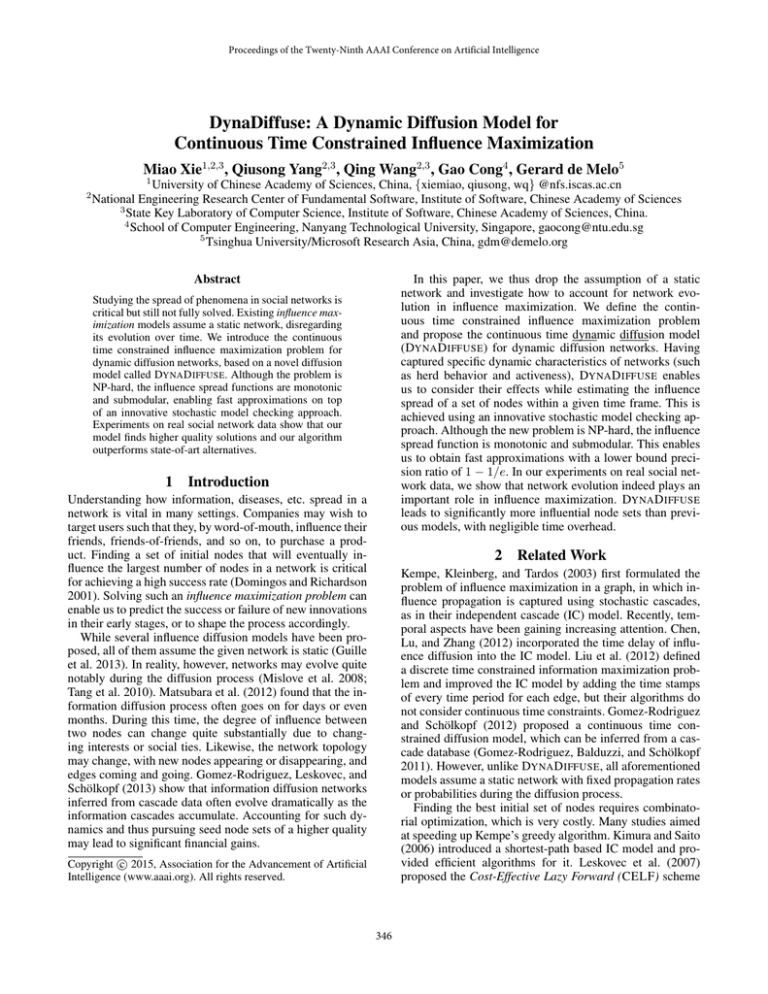
Comparing Models. Figure 3a shows that the seeds’ influence spread obtained by DYNA D IFFUSE (i.e., FastMarginDynamic, CELF-Dynamic) is consistently superior to that
of the static continuous time diffusion model (GomezRodriguez and Schölkopf 2012) (i.e., FastMargin–Static,
CELF–Static), as well as the IC model (Kempe, Kleinberg,
and Tardos 2003) (i.e., CELF-IC). The FAST M ARGIN algorithm is slightly less precise than the pure CELF algorithm
because of its heuristics, but the gap is not large. We additionally compare the DYNA D IFFUSE-estimated influence
spread with the real influence spread in the social network.
To assess the real diffusion, we first crawled all original microblogs published on November 9, 2013 for every user in
the obtained initial set and then calculated the average total number of repostings in the following week (T = 1 to
7). We regard the average total number of repostings as the
influence spread for each user. We only calculate the reposting numbers within our data set (96,700 users) and minus the
overlap. Figure 3b illustrates that the estimated results of our
dynamic model, i.e., FastMargin–Dynamic (Slow, Quick),
are closer to the real situation than those of the static diffusion model, FastMargin–Static. Moreover, the evolution
speed parameters in our model influence the precision of
the estimated results. To get even more precise results, we
could easily tune them with collected historic data. Note
that DYNA D IFFUSE consistently outperforms existing models across different values of these parameters.
120000
100000
80000
60000
40000
20000
0
2
4
6
8
10
12
14
16
18
K, size of initial set
CELF-Dynamic
CELF-Static
FastMargin-Dynamic
FastMargin-Static
CELF-IC
Figure 4: Running time of algorithms (T = 6 days)
Comparing Algorithms. We then evaluated the efficiency
and scalability of DYNA D IFFUSE and the FAST M ARGIN
algorithm. Figure 4 shows running time on a workstation (2.5GHz Dual core, 4GB RAM). FastMargin–Dynamic
and FastMargin–Static are significantly faster than CELF
(CELF–Dynamic and CELF–Static) and are more scalable
as K grows. Interestingly, the time gap between DYNA D IFFUSE (i.e., CELF–Dynamic, FastMargin–Dynamic) and
the static model (i.e., CELF–Static, FastMargin–Static) is
very small. The analysis for DYNA D IFFUSE with FASTM ARGIN is thus just slightly more costly than for the IC
model, yet produces an initial set of significantly higher
quality. Note that FAST M ARGIN’s running time remains almost constant as k increases. CELF-IC has similar behavior,
but with worse output quality, as we have seen earlier.
7
Conclusion and Future Work
We have presented the novel continuous constrained influence maximization problem for dynamic networks, and introduced a novel diffusion model called DYNA D IFFUSE for
it. Under DYNA D IFFUSE, we employ an innovative stochastic model checking approach to considering dynamic effects
and estimating the influence spread of a set of nodes within
a given time frame. Our experiments show that network dynamics indeed have strong effects on the solution’s quality.
In the future, we will investigate how to learn dynamic behavior from data. Additionally, we believe that our novel approach of relying on stochastic model checking can serve as
an important new framework for many new forms of social
network analysis.
351
Acknowledgments
Liu, B.; Cong, G.; Xu, D.; and Zeng, Y. 2012. Time constrained influence maximization in social networks. In Proc.
ICDM, 439 –448.
Liu, B.; Cong, G.; Zeng, Y.; Xu, D.; and Chee, Y. M. 2014.
Influence spreading path and its application to the time constrained social influence maximization problem and beyond.
TKDE 26(8):1904–1917.
Matsubara, Y.; Sakurai, Y.; Prakash, B. A.; Li, L.; and
Faloutsos, C. 2012. Rise and fall patterns of information
diffusion: model and implications. In Proc. SIGKDD, 6–14.
Mislove, A.; Koppula, H. S.; Gummadi, K. P.; Druschel, P.;
and Bhattacharjee, B. 2008. Growth of the flickr social
network. In Proc. WOSN, 25–30.
Raafat, R. M.; Chater, N.; and Frith, C. 2009. Herding in
humans. Trends in cognitive sciences 13(10):420–428.
Tang, J.; Musolesi, M.; Mascolo, C.; and Latora, V. 2010.
Characterising temporal distance and reachability in mobile
and online social networks. SIGCOMM Comput. Commun.
Rev. 40(1):118–124.
Tang, J.; Wu, S.; and Sun, J. 2013. Confluence: Conformity
influence in large social networks. In Proc. SIGKDD, 347–
355.
Tang, Y.; Xiao, X.; and Shi, Y. 2014. Influence maximization: Near-optimal time complexity meets practical efficiency. In Proc. SIGMOD, 75–86.
Viswanath, B.; Mislove, A.; Cha, M.; and Gummadi, K. P.
2009. On the evolution of user interaction in facebook. In
Proc. WOSN, 37–42.
This work is supported by the National Natural Science
Foundation of China under grants 91318301, 91218302,
61432001, 61303163.
References
Alur, R., and Henzinger, T. A. 1999. Reactive modules.
Formal Methods in System Design 15(1):7–48.
Chen, W.; Lu, W.; and Zhang, N. 2012. Time-critical influence maximization in social networks with time-delayed
diffusion process. In Proc. AAAI, 592–598.
Chen, W.; Wang, Y.; and Yang, S. 2009. Efficient influence
maximization in social networks. In Proc. SIGKDD, 199–
208.
Cohen, E.; Delling, D.; Pajor, T.; and Werneck, R. F.
2014. Sketch-based influence maximization and computation: Scaling up with guarantees. In Proc. CIKM, 629–638.
Domingos, P., and Richardson, M. 2001. Mining the network value of customers. In Proc. SIGKDD, 57–66.
Gomez-Rodriguez, M., and Schölkopf, B. 2012. Influence maximization in continuous time diffusion networks.
In Proc. ICML, 313–320.
Gomez-Rodriguez, M.; Balduzzi, D.; and Schölkopf, B.
2011. Uncovering the temporal dynamics of diffusion networks. In Proc. ICML, 561–568.
Gomez-Rodriguez, M.; Leskovec, J.; and Schölkopf, B.
2013. Structure and dynamics of information pathways in
online media. In Proc. WSDM, 23–32.
Guille, A.; Hacid, H.; Favre, C.; and Zighed, D. A. 2013.
Information diffusion in online social networks: a survey.
SIGMOD Rec. 42(1):17–28.
Kempe, D.; Kleinberg, J.; and Tardos, E. 2003. Maximizing
the spread of influence through a social network. In Proc.
SIGKDD, 137–146.
Kimura, M., and Saito, K. 2006. Tractable models for information diffusion in social networks. In Proc. PKDD, 259–
271.
Kossinets, G.; Kleinberg, J.; and Watts, D. 2008. The structure of information pathways in a social communication network. In Proc. SIGKDD, 435–443.
Kwiatkowska, M.; Norman, G.; and Parker, D. 2007.
Stochastic model checking. In Proc. SFM, 220–270.
Kwiatkowska, M.; Norman, G.; and Parker, D. 2011.
PRISM 4.0: Verification of probabilistic real-time systems.
In Proc. CAV, 585–591.
Lang, J., and Wu, S. 2011. Social network user lifetime. In
Proc. ASNAM, 289–296.
Leskovec, J.; Krause, A.; Guestrin, C.; Faloutsos, C.; VanBriesen, J.; and Glance, N. 2007. Cost-effective outbreak
detection in networks. In Proc. SIGKDD, 420–429.
Li, H.; Bhowmick, S. S.; and Sun, A. 2011. Casino: towards
conformity-aware social influence analysis in online social
networks. In Proc. CIKM, 1007–1012.
352