Proceedings of the Thirtieth AAAI Conference on Artificial Intelligence (AAAI-16)
Context-Sensitive Twitter Sentiment Classification Using Neural Network
Yafeng Ren1 , Yue Zhang2 , Meishan Zhang3∗ and Donghong Ji1∗
1. Computer School, Wuhan University, Wuhan, China
2. Singapore University of Technology and Design, Singapore
3. School of Computer Science and Technology, Heilongjiang University, Harbin, China
{renyafeng, dhji}@whu.edu.cn
{yue zhang, meishan zhang}@sutd.edu.sg
Abstract
Sentiment classification on Twitter has attracted increasing research in recent years. Most existing work
focuses on feature engineering according to the tweet
content itself. In this paper, we propose a contextbased neural network model for Twitter sentiment analysis, incorporating contextualized features from relevant Tweets into the model in the form of word embedding vectors. Experiments on both balanced and unbalanced datasets show that our proposed models outperform the current state-of-the-art.
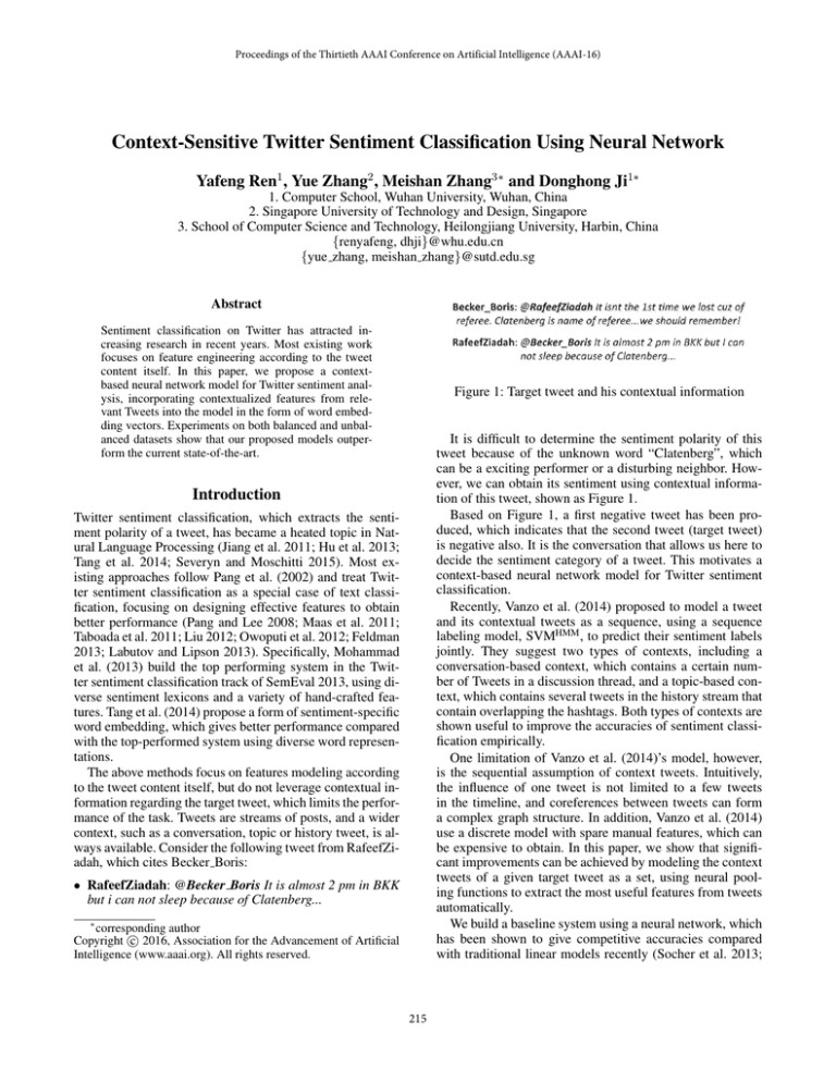
Figure 1: Target tweet and his contextual information
It is difficult to determine the sentiment polarity of this
tweet because of the unknown word “Clatenberg”, which
can be a exciting performer or a disturbing neighbor. However, we can obtain its sentiment using contextual information of this tweet, shown as Figure 1.
Based on Figure 1, a first negative tweet has been produced, which indicates that the second tweet (target tweet)
is negative also. It is the conversation that allows us here to
decide the sentiment category of a tweet. This motivates a
context-based neural network model for Twitter sentiment
classification.
Recently, Vanzo et al. (2014) proposed to model a tweet
and its contextual tweets as a sequence, using a sequence
labeling model, SVMHMM , to predict their sentiment labels
jointly. They suggest two types of contexts, including a
conversation-based context, which contains a certain number of Tweets in a discussion thread, and a topic-based context, which contains several tweets in the history stream that
contain overlapping the hashtags. Both types of contexts are
shown useful to improve the accuracies of sentiment classification empirically.
One limitation of Vanzo et al. (2014)’s model, however,
is the sequential assumption of context tweets. Intuitively,
the influence of one tweet is not limited to a few tweets
in the timeline, and coreferences between tweets can form
a complex graph structure. In addition, Vanzo et al. (2014)
use a discrete model with spare manual features, which can
be expensive to obtain. In this paper, we show that significant improvements can be achieved by modeling the context
tweets of a given target tweet as a set, using neural pooling functions to extract the most useful features from tweets
automatically.
We build a baseline system using a neural network, which
has been shown to give competitive accuracies compared
with traditional linear models recently (Socher et al. 2013;
Introduction
Twitter sentiment classification, which extracts the sentiment polarity of a tweet, has became a heated topic in Natural Language Processing (Jiang et al. 2011; Hu et al. 2013;
Tang et al. 2014; Severyn and Moschitti 2015). Most existing approaches follow Pang et al. (2002) and treat Twitter sentiment classification as a special case of text classification, focusing on designing effective features to obtain
better performance (Pang and Lee 2008; Maas et al. 2011;
Taboada et al. 2011; Liu 2012; Owoputi et al. 2012; Feldman
2013; Labutov and Lipson 2013). Specifically, Mohammad
et al. (2013) build the top performing system in the Twitter sentiment classification track of SemEval 2013, using diverse sentiment lexicons and a variety of hand-crafted features. Tang et al. (2014) propose a form of sentiment-specific
word embedding, which gives better performance compared
with the top-performed system using diverse word representations.
The above methods focus on features modeling according
to the tweet content itself, but do not leverage contextual information regarding the target tweet, which limits the performance of the task. Tweets are streams of posts, and a wider
context, such as a conversation, topic or history tweet, is always available. Consider the following tweet from RafeefZiadah, which cites Becker Boris:
• RafeefZiadah: @Becker Boris It is almost 2 pm in BKK
but i can not sleep because of Clatenberg...
∗
corresponding author
c 2016, Association for the Advancement of Artificial
Copyright Intelligence (www.aaai.org). All rights reserved.
215
output
···
non-linear combination
max
convolution
min
···
pooling
···
···
average
···
···
···
···
···
- +
···
max
···
···
···
···
···
···
average
···
···
pooling
···
···
words
min
···
⊕
···
···
···
···
···
···
words
contextualized features
···
tweet features
Figure 2: The context-based neural network model for Twitter sentiment classification.
this set, ti and tj has the same author. l is the upper limit on
the number of tweets in the posting history of the author for
ti that should be collected.
dos Santos and Gatti 2014; Kalchbrenner, Grefenstette, and
Blunsom 2014). The baseline model takes word embedding
features from the tweet context itself, and performs feature
combination automatically. It gives comparable results to the
best methods in the literature. We further extend the baseline
system with a context-based sub neural network, which extracts important features from context tweets automatically.
In addition to the conversation-based and topic-based contexts proposed by Vanzo et al. (2014), we also investigate a
context based on history tweets of the same author, which
can serve as a prior for a tweet’s sentiment. Results on a
large dataset show that by using such a context-based sub
network, our model can improve two-way sentiment classification performance from 80.68% to 91.33% in macro-F
score.
Topic-based context Let ti ∈ T be a tweet and h(ti ) :
T → P(H) be a function that returns the entire hashtag set
for a tweet ti is
Hi ⊆ H in ti . The topic-based context ΓH,l
i
a set of the most recent l tweets tj such that Hj ∩Hi = ∅ (i.e.
tj and ti share at least one hashtag, and tj has been posted
before ti ).
The Local Sub Network
The local neural network model consists of five layers, including an input layer, a convolutional layer, a pooling layer,
a non-linear combination hidden layer and an output layer.
Input layer Nodes of the input layer denote words in the
tweet in their written order. The neural network model represents words by low-dimensional real-valued vectors. For
each word wi , we use a look-up matrix E to obtain its embedding e(wi ) ∈ RD×1 , where E ∈ RD×V is a model parameter, D is the word vector dimension and V is the vocabulary size. In a typical neural model, E can be randomly initialized, or initialized via distributed word embeddings derived from a large raw corpus.
A Context-based Neural Network Model for
Twitter Sentiment Classification
The proposed model is shown in Figure 2, which has two
main components. The left component is a local-feature sub
neural network, using only local information from the target
tweet itself, while the right component is a contextualized
feature sub network. We study features from conversationbased context, author-based context and topic-based context
about a target tweet, respectively.
Convolution layer The convolution action has been commonly used to synthesize lexical n-gram information (Collobert et al. 2011; dos Santos and Gatti 2014). N-grams have
been shown useful for Twitter sentiment analysis (Mohammad, Kiritchenko, and Zhu 2013; Tang et al. 2014), and we
apply them to our neural network. Given the input layer
e(w1 ) · · · e(wn ), we use the convolution operation to obtain
a new hidden sequence h11 · · · h1n , where,
Context Generation
Conversation-based context For each tweet ti ∈ T , let
r(ti ) : T → T be a function that returns either the tweet
to which ti is a reply, or null if ti is not a reply. Then,
the conversation-based context ΥC,l
of a tweet ti is the sei
quence of tweet iteratively constructed by applying the function r(ti ), until l tweets have been selected or r(ti ) = null,
where l is the maximum size limit for the context.
h1 = tanh(W1 · [e (wi−1 ), e (wi ), e (wi+1 ), 1] ),
i
here e denotes the transpose of the vector e, W1 ∈
RC×(3D+1) is a model parameter, and C is the output dimen-
Author-based context Let ti ∈ T be a tweet, the authoris a set of tweets, such that for ∀i, j in
based context ΩL,l
i
216
pooling
sion. We consider a window size of 3 to combine word embedding features, and use tanh as the activation function for
this hidden layer. With the shared filter upon the word trigrams, independent features are extracted at each position.
Pooling layer We exploit pooling techniques to merge the
varying number of features from the convolution layer into a
vector with fixed dimensions. A typical pooling technique is
the max function, which chooses the highest value on each
dimension from a set of vectors. On the other hand, min and
average pooling have also been used for sentiment classification (Tang et al. 2014; Vo and Zhang 2015), giving significant improvements. We consider all the three pooling methods, concatenating them together as a new hidden layer h2 .
Formally, the values of h2 is defined as:
⎤ ⎡
⎤ ⎡
⎤
⎡
max(h1i1 )
min(h1i1 )
avg(h1i1 ) h2 = ⎣ · · · ⎦ , ⎣ · · · ⎦ , ⎣ · · · ⎦ ,
max(h1iC )
min(h1iC )
original
···
···
⊕
···
···
···
···
···
···
···
···
···
···
···
···
···
···
convolution
characters
Figure 3: Character enhanced word representations.
word representation for both sub networks, obtaining all
word representations by the lookup matrix E. Intuitively,
however, the behavior of contextual words should be different from that of tweet content words. A shared word representation may not capture such differences. Thus we also
consider separated word representations, using different embedding matrixes for the local and contextual sub networks,
which enlarges the model parameter space.
Similar to the local sub network, we use max, min and average pooling to extract features from input words. The features form a real-valued vector with fixed dimension size.
This pooling functions for our contextual model work differently compared with the method of Bamman et al. (2015),
who directly use words as features. Compared with Bamman
et al. (2015), pooling can potentially induce the most important aspects of the salient words, thus offering more useful
information. Note that unlike the local sub network, the contextualized sub network does not use convolution functions,
because the contextualized words are a set, which does not
contain n-gram information.
avg(h1iC )
where h1ij denote the jth dimension of h1i .
Hidden layer Using pooling, we obtain different types of
rich features. In order to fully utilize these sources of information, we use a non-linear hidden layer to automatically
combine the max, min and average pooling features. The
non-linear hidden layer can be computed as:
2
h3 = tanh(W2 · h ),
1
where W2 ∈ RH×(3C+1) is a model parameter, and H is the
dimension of this non-linear hidden layer.
Output layer Finally, an output layer is applied to score
all possible labels according to the features in the last hidden
layer. The output can be computed with a linear transformation using the following equation:
Enhancing Word Representation with Character
Embeddings
o = Wo · h3 ,
N-gram character features have demonstrated their effectiveness in Twitter sentiment analysis (Mohammad, Kiritchenko, and Zhu 2013; dos Santos and Gatti 2014). Some
informative character ngrams can provide useful clues for
the task, such as adverb suffixs “ly” and hashtags “#”. We
propose to use characters to enhance word representation.
For each word, we obtain a dense vector from the lookingup matrix E. Similarly, we also obtain a dense vector from
its characters.
As the Figure 3 shows, we exploit a convolution layer and
a pooling layer to model character sequences, similar to the
local model for word sequences. Each character is denoted
by using a real-valued vector. We use an identical convolution operation to combine a character trigram at each position, obtaining dense representations of the trigrams. The
convolution function is defined by:
where Wo ∈ R2×H is the model parameter for output layer.
The Contextualized Sub Network
We follow Bamman et al. (2015) and extract a set of keywords from different types of contextual information. For
every type of contextual information, we first sort all the
words in the context tweets by their tf-idf values, by regarding the context tweets for a given tweet as one document,
and exploiting all the tweets in the training corpus to generate a number of documents. Then we choose the 100 keywords with the highest tf-idf values as the source of contextualized features.
Given the set of salient words, we build a pooling neural
network, as shown by the right component of Figure 2, combining the output of this pooling layer with the output of the
pooling layer of the local neural model (i.e. the left component), before feeding them to the non-linear hidden layer. In
this way, the hidden layer automatically combines local and
contextualized features.
Similar to the local sub network, we use a real-valued
dense vector to represent each word. We can use a shared
hc = tanh(Wc · [e (ci−1 ), e (ci ), e (ci+1 ), 1] ),
i
where Wc ∈ RCc ×3Dc +1 is a model parameter, and the values
e(·) can be obtained by a looking-up matrix Ec ∈ RDc ×Vc of
characters, where Dc and Vc are the dimension sizes of character vectors and the vocabulary size of characters, respec-
217
tively, and Cc is the output size of the convolution layer. After convolution, we conduct max-pooling to convert the resulting inputs into a fixed-dimension vector1 , and then concatenate the pooling result with the original word representation to form an enhanced representation for each word.
Domain
Unbalanced (P)
Unbalanced (N)
Balanced (P)
Balanced (N)
Training
N
log
i=1
author conversation topic
9,086
561
10,220
5,253
548
5,933
4,784
299
5,365
4,758
481
5,384
Table 1: Corpus statistics, where P and N denote the positive
and negative tweets, respectively.
Our training objective is to minimize the cross-entropy
loss over a set of training examples (xi , yi )|N
i=1 , plus a l2 regularization term,
L(θ) = −
number
11,394
6,606
6,000
6,000
Type
Network structure
eo(yi )
λ
+ θ 2 ,
o
(0)
2
e
+ eo(1)
Training
where θ is the set of model parameters, including E, W1 ,
W2 , Wo , Ec and Wc .
We use online AdaGrad (Duchi, Hazan, and Singer 2011)
to minimize the objective. At step t, the parameters are updated by:
α
gt,i ,
θt,i = θt−1,i − t
2
t =1 gt ,i
#parameter
D = 50, Dc = 10, C =
100, Cc = 30, H = 50
λ = 10−8 , α = 0.01
Table 2: Hyper-parameter values in our model.
We evaluate our models on both balanced and unlabeled
settings. The balanced data include equal numbers of positive and negative tweets, while the ratio of positive and negative tweets in the unbalanced setting is about 2:1. Table
1 shows the corpus statistics of the two datasets. Columns
3-5 represent the subsets of target tweets for which the
author-based context, conversation-based context or topicbased context are available, respectively. The conversationbased context accounts for a very small proportion in all
target tweets. However, more than 85% target tweets have
author-based and topic-based context.
where α is the initial learning rate, and gt,i is the gradient of
the ith dimension at step t.
We follow Glorot et al. (2010) and initialize all the
matrix
and vectorparameters with uniform samples in
(− 6/(r + c), − 6/(r + c)), where r and c are the numbers of rows and columns of the matrixes, respectively. We
assign the initial values of E with pre-trained word embeddings from a large scale tweet corpus.
Evaluation method We perform ten-fold cross-validation
experiments and report the overall performances. The whole
dataset is split into ten equal sections, each decoded by the
model trained from the remaining nine sections. We randomly choose one section from the nine training sections as
the development dataset in order to tune hyper-parameters.
The classification results are measured by macro-F score.
Experiments
Experimental Settings
Data collection We use the Twitter Streaming API2 to collect tweets that express positive (e.g. #happy, #joy), and
negative sentiments (e.g. #sadness, #angry, #frustrated), respectively. Automatic filtering is applied to remove retweets,
duplicates, quotes, spams and tweets written in language
other than English. To address the concern of Davidov et al.
(2010) that tweets with #hashtags between texts are noisy,
we also automatically filter all tweets where the hashtags
are not located at the end of the message.
We remove the #positve (#happy, #joy) and #negative
(#sadness, #angry, #frustrated) hashtags from the tweets,
tagging them as positive and negative examples for training and evaluation, respectively. Finally, we obtain 18,000
tweets that contain 11,394 positive tweets and 6,606 negative tweets. The 18,000 tweets are regarded as basic dataset.
For tweets in the basic dataset, we extract three different
types of contextual tweets by the method described in previous section based on Twitter API. We also remove the #positive and #negative hashtags from the contextual tweets, in
order to avoid predicting sentiment by such explicit clues.
Hyper-parameters There are seven hyper-parameters in
our model, including the network structure parameters (i.e.
the sizes of word vectors D and character vector Dc , the output dimensions of the word convolution layer C and character convolution layer Cc , and the output dimension of the
non-linear combination layer H), and the parameters for supervised training (i.e. the l2 -regularization co-efficient λ and
initial learning ratio α for AdaGrad). The values of the parameters are set according to common values in the machine
learning literature, which are shown in Table 2.
Embeddings The word embeddings are trained on a largescale English tweet corpus that consists of 20 million random tweets crawled by Twitter API, using the word2vec3
tool with default setting. The vocabulary size of word embeddings is 300,000. During training, we use the averaged
vector from the pre-trained word embeddings to initialize
vectors for unknown words. For the vector representation of
characters, we use random initialization, and perform supervised fine-tuning from the training corpus.
1
We do not use min and average pooling here, as our preliminary experiments shows that these two pooling techniques do not
give better performances.
2
http://dev.twitter.com/docs/streaming-apis
3
218
https://code.google.com/p/word2vec
base
+c
+p
83
81
79
77
Balanced
Unbalanced
macro-F Score macro-F Score
Local
83.03
80.90
NRC
82.74
80.24
SSWE
82.97
80.68
+c+p
Model
82
80
78
76
(a) balanced
Table 3: Final results of the local neural model.
(b) unbalanced
base
Figure 4: Influences of different word representations, where
base denotes the word representation with random initialization, +c denotes extension of base by adding character
features, +p denotes extension of base by using pre-trained
word embeddings for initialization and +c+p denotes extension of base by using both +c and +p strategies.
+c
+p
+c+p
92
92
88
88
84
84
shared
separated
(a) balanced
shared
separated
(b) unbalanced
Baseline Methods
Figure 5: The influences of word representations based on
the context-based neural network model, which use the
topic-based context, where base, +c,+p,+c+p have the same
meanings as Figure 4.
We re-implement the following sentiment classification algorithms as the baseline systems:
• NRC: the state-of-art system in the SemEval 2013 Twitter
Sentiment Classification Track, incorporating diverse sentiment lexicons and hand-crafted features (Mohammad,
Kiritchenko, and Zhu 2013).
• SSWE: Tang et al. (2014) propose to learn sentimentspecific word embedding (SSWE) from 10M tweets containing emoticons. They apply SSWE as features for Twitter sentiment classification.
• SVMHMM : Vanzo et al. (2014) model the sentiment classification problem as a sequential classification task over
streams of tweets. SVMHMM is employed to assign sentiment polarities to entire sequences.
methods have positive effect on the overall classification performance, while the max-pooling has the most contribution.
Their combined effect was larger compared with individual
results. The findings are consistent with that of Tang et al.
(2014) and Vo and Zhang (2015), and we omit the detailed
figures due to space limitations.
Comparisons with related work Table 3 shows the final results of our local neural model. Compared with NRC
and SSWE, which are state-of-the-art local models, our local model performs slightly better4 . The above verifies the
effectiveness of our local neural model.
The Local-Feature Neural Network Model
We report results of the neural network model that uses only
local features, which is effectively the model in Figure 2
with the right component being removed. We study the influence of word representations and the effectiveness of rich
pooling functions. The local neural model can later serve as
a baseline system for studying our proposed context-based
neural network model.
The Context-based Neural Network Model
The influence of network configurations We study the
influence of word representations for the context-sensitive
model, focusing on two research questions. First, is it better to use separated word representations for tweet content words and tweet context keywords. The second question is identical to the study of word representations on
the local neural model, including whether improved performances can be achieved via pretrained word embeddings,
and whether they can be achieved via character enhancing.
We use the same pre-trained word embeddings and the same
learning method for character representations for comparisons with the local model, and select the topic-based context as the contextualized features. We observe the same
Influences of word representation Previous work shows
that input word representation is important to a neural network model. We first study the influences of word vector
initialization, by comparing random initialization, the pretrained embeddings and the character-based enhancement.
Figure 4 shows the results on both the balanced and unbalanced datasets. For both datasets, word embeddings with either character-based enhancing or pretraining initialization
can improve the overall performance.
4
The method of Tang et al. (2014) achieves a 80.68% macro-F
score on our unlabeled dataset. Tang et al. (2014) report a macro-F
score of 84.98% on SemEval 2013, which is manually annotated.
One possible reason is that our dataset is built by using distant supervision, there are noisy labels.
Influence of rich pooling functions We empirically compare the effects of the three different pooling techniques,
namely max, min and average pooling, in our local neural network model. Results show that all the three pooling
219
Model
Discussion
Balanced
Unbalanced
macro-F Score macro-F Score
In Table 4, SVMmulti-class represents the baseline system of
Vanzo et al. (2014), which does not utilize any contextual information. Compared with our baseline systems and
local model, it gives lower performance. SVMHMM using
conversation-based context gives macro-F scores of 81.67%
and 79.18% on the balanced and unbalanced datasets, respectively. Our local model obtains 83.03% and 80.90%
macro-F score on the same datasets, respectively. The reasons are two-fold. First, the feature modeling of SVMHMM
use the mixture of bag-of-word, lexical semantic and user
sentiment profile kernel to represent semantic information,
which are spare and less effective compared with word embeddings. SVMmulti-class uses the same feature model, which
partly explains the reason that SVMmulti-class obtains lower
performance. Second, SVMHMM does not use external resources, such as sentiment lexicons, which are proved to be
very effective for NRC (Mohammad, Kiritchenko, and Zhu
2013).
In our context-based neural network model, the three
types of contextual information obtain different performances on both datasets. First, the conversation-based context gives a relatively small improvement in performance
compared with the local neural model. A likely reason is
that the conversation-based context accounts for a very small
proportion in all target tweets. Second, more than 85% target
tweets have the author-based and topic-based context, but
the topic-based context gives much more improvement compared to the author-based context. The main reason is that
author-based contexts express the views and opinions towards some events and people, which may not be relevant to
the target tweet. However, for topic-based contexts, contextual information is closely related to the target tweet. A combination of the three different contexts gives the best performance by utilizing complementary sources of information. In particular, by combining all three sources of contextual features, our model gives 92.27% and 91.33% macro-F
score on both datasets.
For the model of Vanzo et al. (2014), SVMHMM using different types of contextual information can improve 1.11%
and 0.95% macro-F score on average compared with their
baseline system on both datasets, respectively. However, our
context-based model can improve 4.1% and 4.29 macro-F
score on average compared with our local neural system,
respectively. The above demonstrate that the sequential assumption of SVMHMM between one tweet and its contextual tweets is relatively weak, and better performance can be
obtained by modeling a complex graph structure (contextbased neural network) for Twitter sentiment classification.
The Proposed Context-Based Neural Network Model
Local
83.03
80.90
Local+Contextualized (C1)
84.72
82.28∗
Local+Contextualized (C2)
85.13
82.76∗
Local+Contextualized (C3)
91.56
90.53∗
Local+Contextualized (ALL)
92.27
91.33∗
Other Context-Based Models
SVMmulti-class
SVMHMM (C1)
SVMHMM (C2)
SVMHMM (C3)
80.17
81.67
80.86
81.32
77.42
79.18
78.23
78.69
Other Baseline Systems
NRC
SSWE
82.74
82.97
80.24
80.68
Table 4: Final results of our proposed model, where C1, C2
and C3 denotes the conversation-based, author-based and
topic-based context, respectively. ALL represents the mixture of three types of contextual information. The results
with mark ∗ demonstrates that the p-value is below 10−3
using t-test compared with SSWE.
trend when the conversation-based context or author-based
context are used as the contextualized features.
Figure 5 shows the results on both datasets. The separated word representations are better, which gives overall
better results. For the second question, exploiting pre-trained
word embeddings and enhancing embeddings with character
information gives better performance, with separated word
representations. According to the comparisons, we use separated word representation, together with pretrained word
embeddings and character enhancement in the final model.
Final Results Shown in Table 4, the context-based neural
network model gives better performance compared with the
local neural model. The proposed model gives over 90% in
macro-F score using the topic-based context as the contextualized features. For conversation-based context and authorbased context, the performances of context-based model are
slightly higher compared with the local neural model.
Compared with the best local models (SSWE, NRC),
our context-based model can improve about 9% in macroF score when using topic-based model. In addition, our
context-based model by using another two types of contextual information can both outperform the current model.
We also compare the proposed context-based neural
model to the contextualized models of Vanzo et al. (2014),
namely SVMHMM . As Table 4 shows, our proposed neural
network model can improve the macro-F score by 10% compared with sequence labeling method in both the balanced
and the unbalanced settings.
Conclusion
We proposed a context-based neural network model for
Twitter sentiment classification. Compared with previous
work, our neural network model incorporated the features
of tweet content itself and the contextualized features into
a single model in the form of word embedding vectors. Experimental results showed that our proposed context-based
model gave improved performance compared with the state-
220
for Computational Linguistics (ACL), 489–493. Association
for Computational Linguistics.
Liu, B. 2012. Sentiment analysis and opinion mining. Synthesis Lectures on Human Language Technologies 5(1):1–
167.
Maas, A. L.; Daly, R. E.; Pham, P. T.; Huang, D.; Ng, A. Y.;
and Potts, C. 2011. Learning word vectors for sentiment
analysis. In Proceedings of the 49th Annual Meeting of the
Association for Computational Linguistics (ACL), 142–150.
Association for Computational Linguistics.
Mohammad, S. M.; Kiritchenko, S.; and Zhu, X. 2013. Nrccanada: Building the state-of-the-art in sentiment analysis of
tweets. In Second Joint Conference on Lexical and Computational Semantics (* SEM), volume 2, 321–327.
Owoputi, O.; OConnor, B.; Dyer, C.; Gimpel, K.; and
Schneider, N. 2012. Part-of-speech tagging for twitter: Word
clusters and other advances. School of Computer Science,
Carnegie Mellon University, Tech. Rep.
Pang, B., and Lee, L. 2008. Opinion mining and sentiment
analysis. Foundations and trends in information retrieval
2(1-2):1–135.
Pang, B.; Lee, L.; and Vaithyanathan, S. 2002. Thumbs up?:
sentiment classification using machine learning techniques.
In Proceedings of the conference on empirical methods in
natural language processing (EMNLP), 79–86. Association
for Computational Linguistics.
Severyn, A., and Moschitti, A. 2015. Twitter sentiment
analysis with deep convolutional neural networks. In Proceedings of the 38th International Conference on Research
and Development in Information Retrieval (SIGIR), 959–
962. ACM.
Socher, R.; Perelygin, A.; Wu, J. Y.; Chuang, J.; Manning,
C. D.; Ng, A. Y.; and Potts, C. 2013. Recursive deep models for semantic compositionality over a sentiment treebank.
In Proceedings of the conference on empirical methods in
natural language processing (EMNLP), volume 1631, 1642.
Association for Computational Linguistics.
Taboada, M.; Brooke, J.; Tofiloski, M.; Voll, K.; and Stede,
M. 2011. Lexicon-based methods for sentiment analysis.
Computational linguistics 37(2):267–307.
Tang, D.; Wei, F.; Yang, N.; Zhou, M.; Liu, T.; and Qin,
B. 2014. Learning sentiment-specific word embedding for
twitter sentiment classification. In Proceedings of the 52nd
Annual Meeting of the Association for Computational Linguistics (ACL), volume 1, 1555–1565. Association for Computational Linguistics.
Vanzo, A.; Croce, D.; and Basili, R. 2014. A context-based
model for sentiment analysis in twitter. In Proceedings of
the 25th International Conference on Computational Linguistics (COLING), 2345–2354.
Vo, D.-T., and Zhang, Y. 2015. Target-dependent twitter
sentiment classification with rich automatic features. In Proceedings of the Twenty-Fourth International Joint Conference on Artificial Intelligence (IJCAI), 1347–1353.
of-start discrete and continuous word representation models,
demonstrating the effectiveness of context-based neural network model for this task. In addition, we found that under
context-based neural network setting, topic-based contextual
features are the most effective.
Acknowledgements
We thank all reviewers for their detailed comments. This
work is supported by the National Natural Science Foundation of China (No. 61173062, 61373108, 61133012,
61202193), the Major Projects of the National Social Science Foundation of China (No. 11&ZD189), the Key Program of Natural Science Foundation of Hubei, China (Grant
No.2012FFA088), and Singapore Ministry of Education
(MOE) AcRF Tier 2 grant T2MOE201301.
References
Bamman, D., and Smith, N. A. 2015. Contextualized sarcasm detection on twitter. In Ninth International AAAI Conference on Web and Social Media.
Collobert, R.; Weston, J.; Bottou, L.; Karlen, M.;
Kavukcuoglu, K.; and Kuksa, P. 2011. Natural language
processing (almost) from scratch. The Journal of Machine
Learning Research 12:2493–2537.
Davidov, D.; Tsur, O.; and Rappoport, A. 2010. Enhanced
sentiment learning using twitter hashtags and smileys. In
Proceedings of the 23rd International Conference on Computational Linguistics (COLING), 241–249.
dos Santos, C. N., and Gatti, M. 2014. Deep convolutional
neural networks for sentiment analysis of short texts. In Proceedings of the 25th International Conference on Computational Linguistics (COLING), 69–78.
Duchi, J.; Hazan, E.; and Singer, Y. 2011. Adaptive subgradient methods for online learning and stochastic optimization. The Journal of Machine Learning Research 12:2121–
2159.
Feldman, R. 2013. Techniques and applications for sentiment analysis. Communications of the ACM 56(4):82–89.
Glorot, X., and Bengio, Y. 2010. Understanding the difficulty of training deep feedforward neural networks. In International conference on artificial intelligence and statistics,
249–256.
Hu, X.; Tang, J.; Gao, H.; and Liu, H. 2013. Unsupervised
sentiment analysis with emotional signals. In Proceedings
of the 22nd international conference on World Wide Web
(WWW), 607–618.
Jiang, L.; Yu, M.; Zhou, M.; Liu, X.; and Zhao, T. 2011.
Target-dependent twitter sentiment classification. In Proceedings of the 49th Annual Meeting of the Association for
Computational Linguistics (ACL), 151–160. Association for
Computational Linguistics.
Kalchbrenner, N.; Grefenstette, E.; and Blunsom, P. 2014. A
convolutional neural network for modelling sentences. arXiv
preprint arXiv:1404.2188.
Labutov, I., and Lipson, H. 2013. Re-embedding words. In
Proceedings of the 51st Annual Meeting of the Association
221