Proceedings of the Twenty-Ninth AAAI Conference on Artificial Intelligence
Global Policy Construction in Modular Reinforcement Learning
Ruohan Zhang and Zhao Song and Dana H. Ballard
Department of Computer Science, The University of Texas at Austin
2317 Speedway, Stop D9500, Austin Texas 78712-1757 USA
{zharu,zhaos}@utexas.edu dana@cs.utexas.edu
We propose a modular reinforcement learning algorithm which decomposes a Markov decision process
into independent modules. Each module is trained using Sarsa(λ). We introduce three algorithms for forming
global policy from modules policies, and demonstrate
our results using a 2D grid world.
module policies are π1 , · · · , πn . The problem is to form
a global policy π that maximizes global, longterm reward
based on module policies. We assume action space A is
shared among modules. More specifically, for a given global
state s, and module states s1 , · · · , sn , each module selects
its own optimal action a1 , · · · , an according to π1 , · · · , πn .
Our task is to determine global action a∗ for global state s.
Introduction
Our Approach
Reinforcement learning suffers from the curse of dimensionality problem. Such problem limits plain reinforcement
learning algorithms to domains with small state space. Several approaches have been proposed to address this problem, including linear function approximation (Boyan and
Moore 1995), hierarchical reinforcement learning based on
temporal abstraction (Dietterich 1998), and modular reinforcement learning (Doya et al. 2002; Humphrys 1996;
Sprague and Ballard 2003).
Modular reinforcement learning (MRL) utilizes divideand-conquer strategy. It first divides task into smaller, manageable subtasks (modules). Each module will learn its own
policy using reinforcement learning, then module policies
are combined to construct a global policy. MRL approaches
are different in decomposition techniques and global policy construction strategies. In general, an centralized arbitrator is responsible for constructing global policy, and
such problem can introduce additional learning tasks. For
example, arbitrator can use weighted outcome of module policies to determine global policy (Humphrys 1996;
Sprague and Ballard 2003), and weights are learned by their
W-learning algorithm. In this paper we introduce an efficient method that circumvents additional learning problem
and form global policy from module policies.
We construct global policy based on weighted outcomes of
module policies. The critical question is to determine the
weight for all module instances. A simple observation is
made about Q values: for a module at a given state, the variance of Q values across all actions, indicates how indifferent the module is about its action selection. Large variance
indicates that choosing different actions lead to very different expected reward. Let Wi (si ) denote the weight of module i at state si . We choose Wi (si ) = σ(Qi (si , a)), where
σ(Qi (si , a)) is standard deviation of Q values across actions. Then we design three different algorithms for global
policy forming:
Abstract
• Module aggregation algorithm maximizes collective
∗
utility of all modules. Hence we choose
P action a =
arg maxa Q(s, a), where Q(s, a) =
i Qi (si , a). The
idea of this algorithm is originated from (Russell and Zimdars 2003) and (Sprague and Ballard 2003).
• Module selection algorithm maximizes utility of the
module with highest weight. Select module i∗ =
arg maxi Wi (si ), and choose action a∗ = ai .
• Module voting algorithm uses a heuristic similar to
shareholder voting, we let each module to vote for its optimal action, instead of one-module-one-vote, the vote is
weighted. Let K(sP
i , a) be vote count for global action a,
then K(si , a) = i Wi (si ) for all module i whose optimal action ai = a. This is saying that each module i
put Wi (si ) votes on its optimal action ai . Global action
is selected as the action with highest number of votes,
a∗ = arg maxa K(si , a).
Problem Definition
Reinforcement learning problem is often modeled
by a Markov decision process (MDP), which is defined as a tuple hS, A, T, R, γi (Sutton and Barto
1998), we first decompose it into n module MDPs
hS1 , A, T1 , R1 , γ1 i, · · · , hSn , A, Tn , Rn , γn i. Suppose each
module is trained using reinforcement learning and learned
Experiments
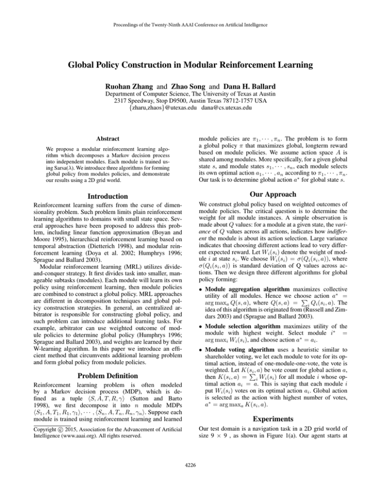
Our test domain is a navigation task in a 2D grid world of
size 9 × 9 , as shown in Figure 1(a). Our agent starts at
c 2015, Association for the Advancement of Artificial
Copyright Intelligence (www.aaai.org). All rights reserved.
4226
the center, and its action space A = {up, down, left, right}.
There are prizes that need to be collected. There are also
cells that are obstacles, stepping onto an obstacle incurs a
negative reward. The dark dot is a predator, starting at upper
left corner of the map, which chases the agent with probability .5 and choose a random action otherwise. Being captured by predator resulted in termination of an experiment
trial and a large negative reward. A trial is successful if agent
collects all prizes within 250 steps, without being captured
by predator. Notice the task domain has state space of size
m2 n
m2
prize
m4 nprize
, with m being the size of grid
nobstacle 2
world and nprize , nobstacle being number of prizes and obstacles. The state space is too large for plain reinforcement
learning algorithms. Our algorithm is as follows:
• Decomposition step. Each object (prize, obstacle, predator) in the grid world is a module. We define three types of
modules: prize collection, obstacle avoidance, and predator escaping. Each type of module is a different reinforcement learning problem with its own MDP. The state
is defined as the relative position (x, y) of an object to
agent. Action spaces are the same for all modules. For reward function, we set Rprize = +10, Robstacle = −10,
Rpredator = −100 for entering the state (0, 0). For discount factor, γprize = .7, γobstacle = 0, γpredator = .1.
Notice that in our domain, there are many modules of the
same type.
• Module training step. By such decomposition, the state
space of the problem is drastically reduced, we train each
type of module using Sarsa(λ) (Sutton and Barto 1998)
with replacing traces. Trained Q tables are stored.
• Navigation and real-time global policy construction step.
During experiment trial, at each global state s, the agent
first calculate module states s1 , · · · , sn for every object.
Then agent uses stored Q tables and one of the global
policy forming algorithm to select global action a∗ and
execute this action and observe new global state s0 . The
loop proceeds until trial terminates.
We compare the performance of our three algorithms with
two baseline algorithms: a random agent and a reflex agent.
The reflex agent chooses the action which maximizes its
one-step-look-ahead reward. Two performance criteria are
average success rate and average number of steps to complete a successful trial. We randomly pick 10% of cells to
contain a prize. Let pobstacle denote the proportion of cells
being obstacle. Since this value defines task difficulty, we
choose pobstacle ∈ [0, .2] with step size of .01, resulted in
21 levels of difficulty. For each level, we randomly generate
103 maps with different layouts, and agent navigates each
map for 5 trials, testing one algorithm per trial. The results
are shown in Figure 1(b) and (c). Our algorithms have higher
success rate and requires fewer steps to success.
(a)
(b)
(c)
Figure 1: (a) Test domain. (b) Success rate. (c) Number of
steps to complete a successful trial.
computed and the effect of discount factor γ. Hence its proposed action is more likely to be selected using Module Selection or Module Voting algorithms. The major advantage
of such approach is that Q tables can be trained beforehand
and stored. Hence during navigation, the computational cost
is the cost of global policy construction algorithm, which is
linear in the number of modules.
In the future, we plan to explore several extensions. First,
to further evaluate the performance of our algorithms, we
need to compare with other approaches to curse of dimensionality problem, such as linear function approximation.
Second, we consider a limitation of current test domain.
Prize, obstacle and predator modules are fairly independent,
their MDPs only share action space. Global policy construction problem could be more challenging when certain degree
of dependency exists between modules, especially when
module state spaces intersect. It is an unanswered question
whether our algorithm can perform well in such a domain.
References
Boyan, J., and Moore, A. W. 1995. Generalization in reinforcement
learning: Safely approximating the value function. In NIPS 369–
376.
Dietterich, T. G. 1998. The maxq method for hierarchical reinforcement learning. In ICML, 118–126. Citeseer.
Doya, K.; Samejima, K.; Katagiri, K.-i.; and Kawato, M. 2002.
Multiple model-based reinforcement learning. Neural computation
14(6):1347–1369.
Humphrys, M. 1996. Action selection methods using reinforcement learning. From Animals to Animats 4:135–144.
Russell, S., and Zimdars, A. 2003. Q-decomposition for reinforcement learning agents. In ICML, 656–663.
Sprague, N., and Ballard, D. 2003. Multiple-goal reinforcement
learning with modular sarsa (0). In IJCAI, 1445–1447.
Sutton, R. S., and Barto, A. G. 1998. Introduction to reinforcement
learning. MIT Press.
Conclusions and Future Work
Recall that for a given module state, we define module
weight to be the standard deviation of Q values across actions. As agent approaches an object, the module weight
of that object becomes larger, due to the way Q values are
4227