Proceedings of the Twenty-Seventh AAAI Conference on Artificial Intelligence
Phase Transition and Network Structure in Realistic SAT Problems
Soumya C. Kambhampati & Thomas Liu
Peggy Payne Academy, McClintock High School, 1830 E Del Rio Dr Tempe, AZ 85282
{budugu2z, thomasliu02}@gmail.com Full report at http://arxiv.org/abs/1304.0145
probability p. This distribution models problems such as
circuit verification, that have loosely coupled clusters of
variables with more constraints among the variables of the
same cluster. Using a SAT solver that we implemented in
Python, we investigated the phase transition behavior of
the SAT instances from these distributions as γ is varied.
Introduction
Previous research (Gomes and Selman 2005) has shown
that 3-SAT problems are easy to solve both when the
“constrainedness” (γ, the ratio of the number of clauses to
the number of variables) is low and when it is high,
abruptly transitioning from easy to hard in a very narrow
region of constrainedness. Most of these “phase transition”
studies were done on SAT instances that follow uniform
random distribution, where variables take part in clauses
with uniform probability, and clauses are independent
(uncorrelated). These assumptions are not satisfied when
we consider SAT instances that result from real problems.
Our project aims for a deeper understanding of the
hardness of SAT problems that arise in practice. We study
two key questions: (1) How does the phase transition
behavior change with more realistic and natural
distributions of SAT problems? and (2) Can we gain an
understanding of the phase transition in terms of the
network structure of these SAT problems? Our hypothesis
is that the network properties help predict and explain how
the easy-to-hard problem transition for realistic SAT
problems differs from that of uniform random distribution.
In aid of the second question, we converted SAT
problems into clausal networks by creating a node for
every variable in the SAT problem, and creating a link
between two nodes if the two variables were found in the
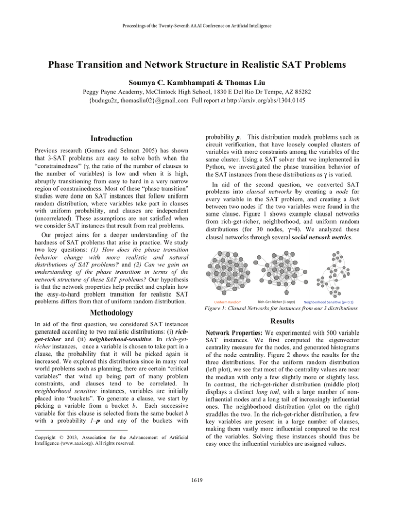
same clause. Figure 1 shows example clausal networks
from rich-get-richer, neighborhood, and uniform random
distributions (for 30 nodes, γ=4). We analyzed these
clausal networks through several social network metrics.
!
" !
Figure 1: Clausal Networks for instances from our 3 distributions
Methodology
Results
In aid of the first question, we considered SAT instances
generated according to two realistic distributions: (i) richget-richer and (ii) neighborhood-sensitive. In rich-getricher instances, once a variable is chosen to take part in a
clause, the probability that it will be picked again is
increased. We explored this distribution since in many real
world problems such as planning, there are certain “critical
variables” that wind up being part of many problem
constraints, and clauses tend to be correlated. In
neighborhood sensitive instances, variables are initially
placed into “buckets”. To generate a clause, we start by
picking a variable from a bucket b. Each successive
variable for this clause is selected from the same bucket b
with a probability 1–p and any of the buckets with
Network Properties: We experimented with 500 variable
SAT instances. We first computed the eigenvector
centrality measure for the nodes, and generated histograms
of the node centrality. Figure 2 shows the results for the
three distributions. For the uniform random distribution
(left plot), we see that most of the centrality values are near
the median with only a few slightly more or slightly less.
In contrast, the rich-get-richer distribution (middle plot)
displays a distinct long tail, with a large number of noninfluential nodes and a long tail of increasingly influential
ones. The neighborhood distribution (plot on the right)
straddles the two. In the rich-get-richer distribution, a few
key variables are present in a large number of clauses,
making them vastly more influential compared to the rest
of the variables. Solving these instances should thus be
easy once the influential variables are assigned values.
Copyright © 2013, Association for the Advancement of Artificial
Intelligence (www.aaai.org). All rights reserved.
1619
""+*
""+$
""*(
""*"
"")&
""(*
""($
""'(
""'"
""&&
""%*
""%$
""$(
""$"
!"(!
!"&*
!"%*
!"$*
!"#)
!"")
!"!(
!!*(
!!)(
!!('
!!''
!!&&
!!%&
!!$&
!!#%
!
!!"%
#!
%'
%"
$'
$"
#'
#"
'
"
""#&
%!
"""*
'!
!!!$
)!
!!*#
!!)'
!!)"
!!(&
!!'*
!!'%
!!&)
!!&$
!!%(
!!%"
!!$'
!!$!
!!#%
!!"*
!!"$
!!!)
"!!
!!!#
$&
$!
#&
#!
"&
"!
&
!
variables. We found (Figure 4) that the distribution does
exhibit phase transition, but the transition occurs at around
γ=2.8, which is significantly lower than the phase
transition point γ=4.3 for uniform random distribution.
This can be explained in terms of its network properties
(Figures 2 and 3). As shown by the long-tailed node
centrality in Figure 2 middle plot, clauses in the rich-getricher distribution are centered on a smaller set of
variables. Satisfiability drops earlier because the high
concentration of clauses surrounding certain variables
raises the chances of unsatisfiability. To test this
hypothesis, we increased the probability of rich getting
richer (instead of adding one copy of the chosen variable
back into the selection pool, we add larger number of
copies). As shown by the right plot in Figure 4, this makes
the transition occur at even lower γ values. The satisfiable
problems are also solved faster--once the few key variables
around which the problem is centered are determined, the
rest fall into place through unit propagation.
For the neighborhood distribution as p is varied from 1
to 0, we note (Figure 5, right plot) that the phase transition
occurs earlier, and the median number of backtracks drops
significantly. This is because as p goes to zero, the SAT
problem gets increasingly localized into several smaller,
distinct problems (as confirmed by its high average
clustering coefficient, its characteristically small path
length, and its high proximity ratio; Figure 3). The rate of
satisfiability (Figure 5, left plot) also drops earlier with
smaller p values. This is because with several smaller
problems, only one local problem has to be unsatisfiable
for the entire problem to be unsatisfiable. Furthermore,
each smaller problem, with a correspondingly smaller
neighborhood of variables to choose from, is more
constrained, and thus requires fewer clauses to achieve the
same amount of constrainedness.
'""
&!!
"""$
&!!
Figure 2: Histogramss off the eigenvector centralities
ceentralities of variables
in 500-variable SAT instances (with γ = 4.3) drawn from uniform
random (left), rich-get-richer (center) and neighborhood (right).
%
$
#
"
!
!
!
!
"
$
Figure 3: Avg. clustering coefficient, avg. length, and proximity
ratio in 50 variable SAT instances with uniform random (orange),
rich-get-richer (gray) and neighborhood (blue) distributions
!
!
"
#
%
!
!%
"
"%
#
#%
$
$%
%
%%
&
&%
'
'%
(
γ
Figure 4: Phase transition behavior for “rich-get-richer.” The
left plot shows the transition point shifting left as the number of
copies increase.
Figure 5: Phase transition point for “neighborhood-sensitive”
shifts left as p is varied from 1 (uniform random) to 0.
Figure 3 shows the results for the clustering coefficient,
average length and proximity ratio. We see that for any
given value of γ, the rich-get-richer and neighborhood
distributions produce SAT instances with more clustered
clausal networks. The average path length at any γ is
significantly lower for the neighborhood distribution. Since
variables become more connected within their
neighborhoods, path length between nodes inside a
neighborhood reduces. The right plot in Figure 3 shows
the proximity ratio (Walsh 1999), which compares the ratio
of the network’s clustering coefficient and average length
to the corresponding ratio of a uniform random network
(thus it is always 1 for uniform random). The
neighborhood distribution shows a high proximity ratio
because it has a higher clustering coefficient and a lower
average length. Thus it conforms to the idea of a “small
world” network as several loosely connected clusters
(Watts and Strogatz 1998). Rich-get-richer distribution
also has a higher proximity ratio (especially for low γ
values), but not as pronounced as the neighborhood one.
Phase Transition Behavior: We solved random SAT
instances from rich-get-richer distribution with 150
Conclusion
Our analysis of rich-get-richer and neighborhood
distributions showed that they reach the transition point at
lower constrainedness values, in comparison to uniform
random distribution. We also showed that this shift can be
explained in terms of the small-world properties of their
clausal networks. In future, we hope to examine the
predictive power of these insights on instances from
planning and circuit verification problems.
Acknowledgements: We thank the members of the ASU
Data Mining & Machine Learning lab, Will Cushing, and
Prof. Bart Selman for helpful comments. We also thank the
Army Research Office High School Apprenticeship
Program for internship support at the ASU DMML lab.
References
Gomes, C.P., and Selman, B. 2005. Can Get Satisfaction. Nature.
Walsh, T. 1999. Search in a Small World. IJCAI.
Watts, D.J., and Strogatz, S.H. 1998. Collective Dynamics of
“Small World” Networks. Nature. 393:440-442.
1620