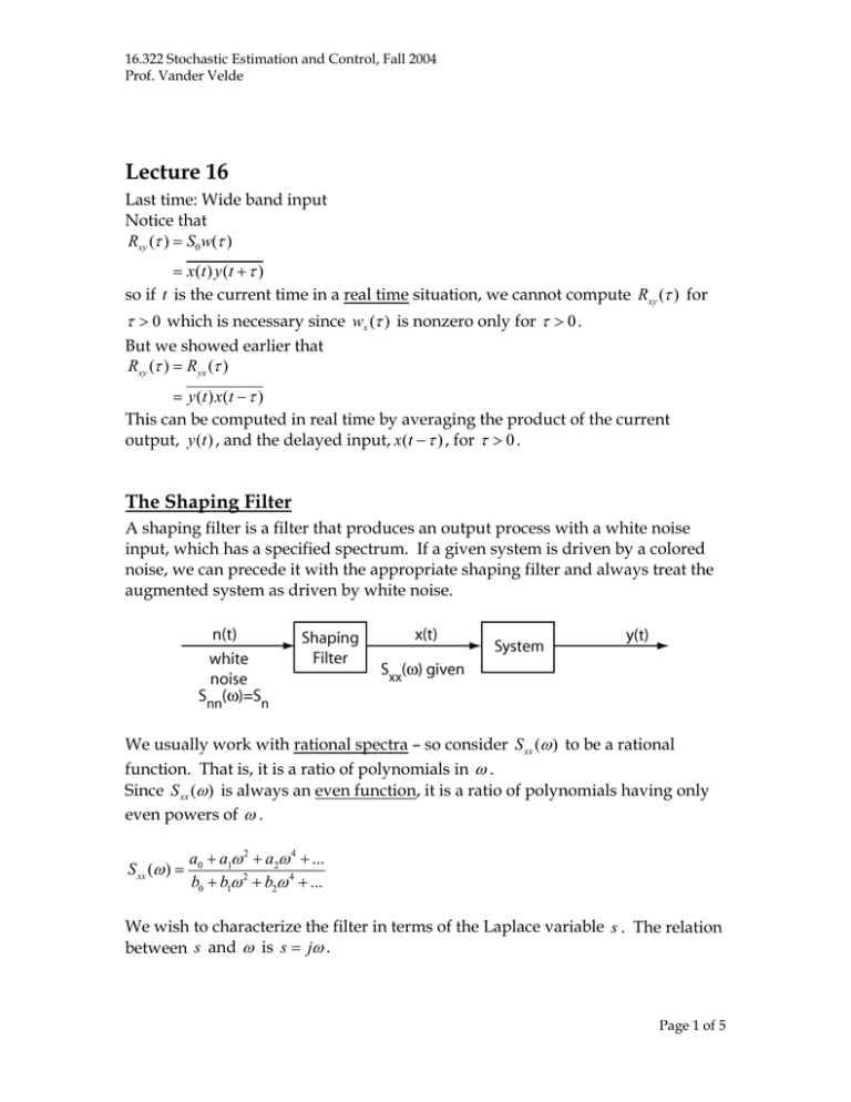
16.322 Stochastic Estimation and Control, Fall 2004
Prof. Vander Velde
Lecture 16
Last time: Wide band input
Notice that
Rxy (τ ) = S0 w(τ )
= x (t ) y (t + τ )
so if t is the current time in a real time situation, we cannot compute Rxy (τ ) for
τ > 0 which is necessary since wx (τ ) is nonzero only for τ > 0 .
But we showed earlier that
Rxy (τ ) = R yx (τ )
= y (t ) x (t − τ )
This can be computed in real time by averaging the product of the current
output, y (t ) , and the delayed input, x (t − τ ) , for τ > 0 .
The Shaping Filter
A shaping filter is a filter that produces an output process with a white noise
input, which has a specified spectrum. If a given system is driven by a colored
noise, we can precede it with the appropriate shaping filter and always treat the
augmented system as driven by white noise.
We usually work with rational spectra – so consider S xx (ω ) to be a rational
function. That is, it is a ratio of polynomials in ω .
Since S xx (ω ) is always an even function, it is a ratio of polynomials having only
even powers of ω .
S xx (ω ) =
a0 + a1ω 2 + a2ω 4 + ...
b0 + b1ω 2 + b2ω 4 + ...
We wish to characterize the filter in terms of the Laplace variable s . The relation
between s and ω is s = jω .
Page 1 of 5
16.322 Stochastic Estimation and Control, Fall 2004
Prof. Vander Velde
Rewrite S xx in terms of s . Since only even powers of ω appear there will be no
imaginary terms.
ω 2 = −s2
ω 4 = + s4
ω 6 = − s6
etc.
a0 − a1s 2 + a2 s 4 − a3s 6 ...
S xx ( s ) =
b0 − b1s 2 + b2 s 4 − b3s 6 ...
Factor the numerator and denominator in terms of s 2 .
S xx
(s
( s) = c
(s
2
2
− c1 )( s 2 − c2 ) ...
− d1 )( s 2 − d1 ) ...
The poles and zeroes are located at:
Zeroes at s = ± ci , where i = 1, 2,...
Poles at s = ± d i , where i = 1, 2,...
If ci is real and positive, then
ci is real
If ci is real and negative, then
ci is purely imaginary
This kind of root always appears with even multiplicity.
( s 2 − ci ) → ( −ω 2 − ci )
Notice that in terms of ω , this must be true to avoid a change of sign of S xx (ω ) .
For small ω , ( −ω 2 − ci ) is positive.
For large ω , ( −ω 2 − ci ) is negative.
If ci is complex, then ci* is another root.
The poles or zeroes are at:
⎧ + ci = + a + jb
⎪
⎪⎪ − ci = − a − jb
s=⎨
*
⎪ + ci = + a − jb
⎪
*
⎪⎩ − ci = − a + jb
Page 2 of 5
16.322 Stochastic Estimation and Control, Fall 2004
Prof. Vander Velde
Collect the factors which define poles or zeroes in the left-half plane together
with the square root of any factorable constant ( c ). Call the product S xx ( s ) L the left hand factor of the spectrum.
Collect the remaining factors, which define poles or zeroes in the right-half
plane, together with the square root of the factorable constant. Call the product
S xx ( s ) R - the right hand factor of the spectrum.
Then:
S xx ( s ) = S xx ( s ) L S xx ( s ) R
From the symmetry of the pole-zero pattern, we can see that
S xx ( s ) R = S xx ( − s ) L
Call the shaping filter transfer function F ( s ) . The input-output relation for
power spectral density functions in terms of s is
S xx ( s ) = F ( s ) F ( − s ) Snn ( s )
But with S xx ( s ) factored and n(t ) white,
S xx ( s ) L S xx ( s ) R = F ( s ) F ( − s ) Sn
S xx ( s ) L S xx ( − s ) L = F ( s ) F ( − s ) Sn
One solution for F ( s ) which produces the desired output spectrum is
1
F ( s) =
S xx ( s ) L
Sn
We can choose Sn to be 1 if we wish.
By construction, this filter is stable and minimum phase.
If Snn (ω ) is not broadband relative to the system,
Page 3 of 5
16.322 Stochastic Estimation and Control, Fall 2004
Prof. Vander Velde
F ( s) =
S xx ( s ) L
Snn ( s ) L
Example
Suppose a disturbance process has a spectrum with the following shape.
Suppose this function is well approximated by
10ω 2
S xx (ω ) = 4
ω + 5ω 2 + 4
Then:
−10s 2
S xx ( s ) = 4
s − 5s 2 + 4
10 s( − 10 s )
= 2
( s − 1)( s 2 − 4)
⎡
⎤⎡
⎤
10 s
10 s
=⎢
⎥⎢
⎥
( s + 1)( s + 2) ⎦ ⎣ ( s − 1)( s − 2) ⎦
⎣14
42443 1442443
S xx ( s ) L
S xx ( s ) R
With unit intensity noise driving the shaping filter, the filter transfer function
is
10 s
10 s
F ( s) =
= 2
( s + 1)( s + 2) s + 3s + 2
If you are going to work in terms of a state space model, you would now have to
define a state variable realization of this transfer, and augment the state space
model of the original system with it.
Page 4 of 5
16.322 Stochastic Estimation and Control, Fall 2004
Prof. Vander Velde
General Introduction to Filtering and Control System Design
Suppose you have input data up to time t , and at that time you want to produce
a smoothed estimate of the signal (which is a real time operation). This called
filtering.
Suppose you want an estimate of a signal at time t + τ in the future. This is
called predicting.
Suppose you want an estimate of a signal at time t − τ in the past, using data
available up to time t . This is called smoothing.
Ground rules
We shall treat in a fairly general manner the problem of optimum design of
systems under the following conditions:
1. The system is assumed to be linear and physically realizable.
2. The inputs to the system (e.g., signals, noise, disturbances), are members of
stationary random processes.
3. The desired operation of the system is a linear time-invariant operation on the
signal.
4. The optimum system is defined to be that which yields the minimum steady
state mean squared error between actual output and derived output.
With stationary inputs, the input correlation functions are invariant with time;
these are the invariants which are the basis for prediction.
Thus we shall be finding the realizable linear system which operating on the
signal and noise yields an output which best approximates in the mean squared
sense the output of an ideal linear operator, not necessarily realizable, operating
on the signal only. We shall find optimum systems in two senses:
1. Configuration fixed – find optimum parameter values
2. Configuration semi-free – find best linear realizable compensator
a. Configuration free – find best linear realizable system
Page 5 of 5