16.322 Stochastic Estimation and Control, Fall 2004
Prof. Vander Velde
Lecture 20
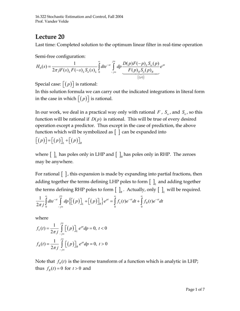
Last time: Completed solution to the optimum linear filter in real-time operation
Semi-free configuration:
j∞
∞
1
D ( p ) F ( − p ) L Sis ( p ) pt
− st
H 0 ( s) =
dte ∫ dp
e
∫
2π jF ( s ) L F ( − s ) L Sii ( s ) L 0
F ( p ) R Sii ( p ) R
− j∞
144424443
⎡⎣( p )⎤⎦
Special case: ⎡⎣ ( p )⎤⎦ is rational:
In this solution formula we can carry out the indicated integrations in literal form
in the case in which ⎡⎣ ( p )⎤⎦ is rational.
In our work, we deal in a practical way only with rational F , Sis , and Sii , so this
function will be rational if D ( p ) is rational. This will be true of every desired
operation except a predictor. Thus except in the case of prediction, the above
function which will be symbolized as [ ] can be expanded into
⎡⎣ ( p )⎤⎦ = ⎡⎣( p )⎤⎦ L + ⎡⎣ ( p )⎤⎦ R
where
[ ]L
has poles only in LHP and
[ ]R has poles only in RHP.
The zeroes
may be anywhere.
[ ] , this expansion is made by expanding into partial fractions, then
adding together the terms defining LHP poles to form [ ]L and adding together
the terms defining RHP poles to form [ ]R . Actually, only [ ]L will be required.
For rational
1
∞
j∞
dte ∫
2π j ∫
− st
− j∞
0
{
}
∞
∞
dp ⎡⎣( p )⎤⎦ L + ⎡⎣( p )⎤⎦ R e = ∫ f L (t )e dt + ∫ f R (t )e − st dt
pt
0
− st
0
where
f L (t ) =
f R (t ) =
1
j∞
∫ ⎡⎣( p )⎤⎦
2π j − j∞
1
L
e pt dp = 0, t < 0
j∞
∫ ⎡⎣( p )⎤⎦
2π j − j∞
R
e pt dp = 0, t > 0
Note that f R (t ) is the inverse transform of a function which is analytic in LHP;
thus f R (t ) = 0 for t > 0 and
Page 1 of 7
16.322 Stochastic Estimation and Control, Fall 2004
Prof. Vander Velde
∞
∫f
R
(t )e − st dt = 0
0
Also f L (t ) is the inverse transform of a function which is analytic in RHP; thus
f L (t ) = 0 for t < 0 . Thus
∞
∫
0
f L (t )e − st dt =
∞
∫
−∞
f L (t )e − st dt = ⎡⎣( s )⎤⎦ L
Thus finally,
⎡ D ( s ) F ( − s ) L Sij ( s ) ⎤
⎢ F ( s) S ( s)
⎥
R ii
R
⎣
⎦L
H 0 ( s) =
F ( s ) L F ( − s ) L Sii ( s ) L
In the usual case, F ( s ) is a stable, minimum phase function. In that case,
F ( s ) L = F ( s ) , F ( s ) R = 1 ; that is, all the poles and zeroes of F ( s ) are in the LHP.
Similarly, F ( − s ) L = 1 . Then
⎡ D ( s ) Sij ( s ) ⎤
⎢ S ( s) ⎥
H 0 ( s ) = ⎣ ii R ⎦ L
F ( s ) Sii ( s ) L
Thus in this case the optimum transfer function from input to output is
⎡ D ( s ) Sij ( s ) ⎤
⎢ S ( s) ⎥
F ( s ) H 0 ( s ) = ⎣ ii R ⎦ L
Sii ( s ) L
and the optimum function to be cascaded with the fixed part is obtained from
this by division by F ( s ) , so that the fixed part is compensated out by
cancellation.
Free configuration problem:
⎡ D ( s ) Sij ( s ) ⎤
⎢ S ( s) ⎥
H 0 ( s ) = ⎣ ii R ⎦ L
Sii ( s ) L
Optimum free configuration filter:
Page 2 of 7
16.322 Stochastic Estimation and Control, Fall 2004
Prof. Vander Velde
We started with a closed-loop configuration:
”
C ( s)
1 + C ( s) F ( s ) B( s )
H ( s)
C ( s) =
1 − H ( s) F ( s) B( s)
H ( s) =
The loop will be stable, but C ( s ) may be unstable.
Special comments about the application of these formulae:
a) Unstable F ( s ) cannot be treated because the Fourier transform of wF (t )
does not converge in that case. To treat this system, first close a feedback
loop around F ( s ) to create a stable “fixed” part and work with this stable
feedback system as F ( s ) . When the optimum compensation is found, it
can be collected with the original compensation if desired.
b) An F ( s ) which has poles on the jω axis is the limiting case of functions
for which the Fourier transform converges. You can move the poles just
into the LHP by adding a real part +ε to the pole locations. Solve the
problem with this ε and at the end set it to zero.
Zeroes of F ( s ) on jω axis can be included in either factor and the result
will be the same. This will permit cancellation compensation of poles of
F ( s ) on the jω axis, including poles at the origin.
c) In factoring Sii ( s ) into Sii ( s ) L Sii ( s ) R , any constant factor in Sii ( s ) can be
divided between Sii ( s ) L and Sii ( s ) R in any convenient way. The same is
true of F ( s ) and F ( − s ) .
d) Problems should be well-posed in the first place. Avoid combinations of
D ( s ) and S ss (ω ) which imply infinite d (t ) 2 because that may assume
infinite e 2 for any realizable filter. Such as a differentiator on a signal
1
which falls off as 2 .
ω
e) The point at t = 0 was left hanging in several steps of the derivation of the
solution formula. Don’t bother checking the individual steps; just check
the final solution to see if it satisfies the necessary conditions.
Page 3 of 7
16.322 Stochastic Estimation and Control, Fall 2004
Prof. Vander Velde
The Wiener-Hopf equation requires l (τ 1 ) = 0 for τ 1 ≥ 0 . Thus L( s ) should be
1
analytic in LHP and go to zero at least as fast as for large s .
s
L( s ) = F ( − s ) H 0 ( s ) F ( s ) Sii ( s ) − F ( − s ) D ( s ) Sis ( s )
We have solved the problem of the optimum linear filter under the least mean
squared error criterion.
Further analysis shows that if the inputs, signal and noise, are Gaussian, the
result we have is the optimum filter. This is, there is no filter, linear or nonlinear
which will yield smaller mean squared error.
If the inputs are not both Gaussian, it is almost sure that some nonlinear filters
can do better than the Wiener filter. But theory for this is only beginning to be
developed on an approximate basis.
Note that if we only know the second order statistics of the inputs, the optimum
linear filter is the best we can do. To take advantage of nonlinear filtering we
must know the distributions of the inputs.
Example: Free configuration predictor (real time)
A
a − s2
Snn ( s ) = Sn
The s, n are uncorrelated.
S ss ( s ) =
2
D ( s ) = e sT
Page 4 of 7
16.322 Stochastic Estimation and Control, Fall 2004
Prof. Vander Velde
Use the solution form
∞
j∞
∞
j∞
1
D ( p ) Sis ( p ) pt
H 0 ( s) =
dte − st ∫ dp
e
∫
2π jSii ( s ) L 0
Sii ( p ) R
− j∞
1
S ( p ) p ( t +T )
dte − st ∫ dp is
e
=
∫
2π jSii ( s ) L 0
Sii ( p ) R
− j∞
Sii ( s ) = S ss ( s ) + Snn ( s )
A
+ Sn
a + s2
⎡ A
2
2⎤
⎢S +a −s ⎥
= Sn ⎢ n 2 2 ⎥
⎢ a −s
⎥
⎣⎢
⎦⎥
=
2
b2 − s 2
a2 − s2
⎡ b + s⎤⎡b − s⎤
= ⎢ Sn
⎣ a + s ⎥⎦ ⎢⎣ a − s ⎥⎦
= Sn
where b2 = a 2 +
A
.
Sn
A
( a + s )( a − s )
Sis ( p )
A( a − s )
=
Sii ( p ) R (a + s )( a − s )(b − s )
Sis ( p ) = S ss ( p ) =
A
(a + s )(b − s )
A
A
= b+a + a+b
a+s b−s
=
Using the integral form,
A
⎧ A − a ( t +T )
j∞
, t > −T
1
a + b e p ( t +T ) dp = ⎪ a + b e
⎨
∫
2π j − j∞ p + a
⎪⎩0, otherwise
Page 5 of 7
16.322 Stochastic Estimation and Control, Fall 2004
Prof. Vander Velde
A
⎧ A b ( t +T )
, t < −T
a + b e p ( t +T ) dp = ⎪ a + b e
⎨
∫
2π j − j∞ b − p
⎪⎩0, otherwise
1
∞
− st
∫e
0
j∞
∞
A − a ( t +T )
A − aT − ( s + a ) t
e
dT =
e ∫e
dt
a+b
a+b
0
=
H 0 ( s) =
A − aT 1
e
a+b
s+a
A − aT
(s + a)
Ae − aT
1
e
=
a+b
( s + a ) S n ( s + b) S n ( a + b) s + b
where b = a 2 +
A
.
Sn
Note the bandwidth of this filter and the gain ~ e − aT which is the correlation
between S (t ) and S (t + T )
Example: Semi-free problem with non-minimum phase F . Optimum
compensator
F ( s) = K
(c − s)
s (d + s)
A
a − s2
Snn ( s ) = Sn
The s, n are uncorrelated.
S ss ( s ) =
2
Servo example where we’d like the output to track the input, so the desired
operator, D ( s ) = 1 .
Page 6 of 7
16.322 Stochastic Estimation and Control, Fall 2004
Prof. Vander Velde
b2 − s 2
Sii ( s ) = Sn 2 2
a −s
b+s
Sii ( s ) L = Sn
a+s
b−s
Sii ( s ) R = Sn
a−s
K
F ( s)L =
( s + ε )( d + s )
F ( s) R = c − s
F ( − s) = K
c+s
(ε − s )( d − s )
F ( − s) L = c + s
⎡⎣ ( s )⎤⎦ =
=
D ( s ) F ( − s ) L Sis ( s )
F ( s ) R Sii ( s ) R
A(c + s)
(c + s ) A(a − s )
=
( a + s )( a − s )( c − s )( b − s ) ( a + s )( c − s )( b − s )
Page 7 of 7