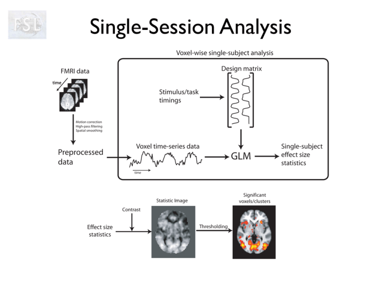
Single-Session Analysis
Voxel-wise single-subject analysis
Design matrix
FMRI data
time
Stimulus/task
timings
Motion correction
High-pass filtering
Spatial smoothing
Preprocessed
data
Voxel time-series data
GLM
time
Significant
voxels/clusters
Statistic Image
Contrast
Effect size
statistics
Thresholding
Single-subject
effect size
statistics
Ti
m
e
Two different views of the data
...
A “smallish”
number of
volumes
A large
number of
time series
FMRI Modelling and Statistics
•
•
•
•
•
•
An example experiment
Multiple regression (GLM)
T and F Contrasts
Null hypothesis testing
The residuals
Thresholding: multiple comparison
correction
FMRI Modelling and Statistics
•
•
•
•
•
•
An example experiment
Multiple regression (GLM)
T and F Contrasts
Null hypothesis testing
The residuals
Thresholding: multiple comparison
correction
An example experiment
An FMRI adaptation of a classical PET experiment
• Three types of events
• 1st type: Word Generation
Healthy
Volunteer
+
Screen
Scanner
Bed
An example experiment
An FMRI adaptation of a classical PET experiment
• Three types of events
• 1st type: Word Generation
Verb is generated
Catch
Noun is presented
Healthy
Volunteer
Jellyfish
Screen
Scanner
Bed
An example experiment
An FMRI adaptation of a classical PET experiment
• Three types of events
• 1st type: Word Generation
Verb is generated
Fry
Noun is presented
Healthy
Volunteer
Burger
Screen
Scanner
Bed
An example experiment
An FMRI adaptation of a classical PET experiment
• Three types of events
• 1st type: Word Generation
• 2nd type: Word Shadowing
Verb is repeated
Swim
Verb is presented
Healthy
Volunteer
Swim
Screen
Scanner
Bed
An example experiment
An FMRI adaptation of a classical PET experiment
• Three types of events
• 1st type: Word Generation
• 2nd type: Word Shadowing
Verb is repeated
Giggle
Verb is presented
Healthy
Volunteer
Giggle
Screen
Scanner
Bed
An example experiment
An FMRI adaptation of a classical PET experiment
•
•
•
•
Three types of events
1st type: Word Generation
2nd type: Word Shadowing
3rd type: Null event
Crosshair is shown
Healthy
Volunteer
+
Screen
Scanner
Bed
An example experiment
An FMRI adaptation of a classical PET experiment
•
•
•
•
Three types of events
1st type: Word Generation
2nd type: Word Shadowing
3rd type: Null event
Crosshair is shown
z
z
z
z
z
Healthy
Volunteer
+
Screen
Scanner
Bed
z
z
z
zz
An example experiment
An FMRI adaptation of a classical PET experiment
•
•
•
•
•
Three types of events
1st type: Word Generation
2nd type: Word Shadowing
3rd type: Null event
6 sec ISI, random order
Healthy
Volunteer
+
Screen
Scanner
Bed
An example experiment
An FMRI adaptation of a classical PET experiment
•
•
•
•
•
•
Three types of events
1st type: Word Generation
2nd type: Word Shadowing
3rd type: Null event
6 sec ISI, random order
For 24 events of each type
Giggle
Swim
Fry
Catch
Healthy
Volunteer
Swim
+
Jellyfish
Burger
Giggle
Etc...
Screen
Scanner
Bed
FMRI Modelling and Statistics
•
•
•
•
•
•
An example experiment
Multiple regression (GLM)
T and F Contrasts
Null hypothesis testing
The residuals
Thresholding: multiple comparison
correction
Building a model
Our task is now to build a model for that experiment
What is our predicted response to the word generation
events?
Building a model
Our task is now to build a model for that experiment
What is our predicted response to the word generation
events?
Stick-function at each occurrence
of a “generation event”
...
First 100 seconds
Well, hardly like this...
Building a model
Our task is now to build a model for that experiment
What is our predicted response to the word generation
events?
=
⊗
First 100 seconds
=
HRF
predicted response
First 100 seconds
That looks better!
Building a model
Our task is now to build a model for that experiment
What is our predicted response to the word generation
events?
=
⊗
445 seconds
HRF
=
445 seconds
And this is the prediction for the whole time-series
Building a model
Our task is now to build a model for that experiment
What is our predicted response to the word generation
events?
+
prediction
445 seconds
So, if we spot a time-series like this
Building a model
Our task is now to build a model for that experiment
What is our predicted response to the word generation
events?
+
prediction
445 seconds
And then check it against our prediction
we can conclude that this pixel is into word generation
Building a model
Our task is now to build a model for that experiment
And we can do the same for the word shadowing
events?
⊗
=
445 seconds
=
prediction
445 seconds
This time we used the onset times for the shadowing
events to get the predicted brain response for those
Building a model
Our task is now to build a model for that experiment
And we can do the same for the word shadowing
events?
+
prediction
445 seconds
And we can look for voxels that match that
Formalising it: Multiple regression
Word
Generation
+
Word
Shadowing
Unknown
“parameters”
≈ β1·
Observed data
+ β2·
Predicted responses
“Regressors”
Slight detour: Making regressors
Event timings at
“high” resolution
⊗
Convolve with
HRF
Predictions at
“high” resolution
Sub-sample at TR
of experiment
Regressor
Estimation:
Finding the “best” parameter values
• The estimation entails finding the parameter values such
that the linear combination ”best” fits the data.
+
Word
Generation
≈ β1·
Let’s try
these
parameter
values
0.5
Word
Shadowing
+ β2·
0.5
Estimation:
Finding the “best” parameter values
• The estimation entails finding the parameter values such
that the linear combination ”best” fits the data.
+
Word
Generation
≈ β1·
0.5
Hmm, not a
great fit
Word
Shadowing
+ β2·
0.5
Estimation:
Finding the “best” parameter values
• The estimation entails finding the parameter values such
that the linear combination ”best” fits the data.
+
Oh dear,
even worse
Word
Generation
Word
Shadowing
≈ β1·
+ β2·
0
1
Estimation:
Finding the “best” parameter values
• The estimation entails finding the parameter values such
that the linear combination ”best” fits the data.
+
But that looks
good
Word
Generation
Word
Shadowing
≈ β1·
+ β2·
1.04
-0.10
Estimation:
Finding the “best” parameter values
• The estimation entails finding the parameter values such
that the linear combination ”best” fits the data.
+
≈ β1·
+ β2·
1.10
1.02
And different voxels yield different parameters
Estimation:
Finding the “best” parameter values
• The estimation entails finding the parameter values such
that the linear combination ”best” fits the data.
+
≈ β1·
+ β2·
-0.04
-0.03
And different voxels yield different parameters
One model to fit them all
Ti
me
1
1.10
1.02
/stats/pe1
2
/stats/pe2
1.04
.10
Model
.04
.03
And we can also estimate the residual
error
Difference between data and
best fit: “Residual error”
Residual errors
And we can also estimate the residual
error
Ti
me
1
1.10
1.02
/stats/pe1
2
/stats/pe2
1.04
.10
2
Model
.04
.03
/stats/
sigmasquareds
Summary of what we learned so far
• The “Model” consists of a set of “regressors” i.e. tentative
time series that we expect to see as a response to our
stimulus
• The model typically consists of our stimulus functions
convolved by the HRF
• The estimation entails finding the parameter values such
that the linear combination of regressors ”best” fits the
data
• Every voxel has its own unique parameter values, that is
how a single model can fit so many different time series
• We can also get an estimate of the error through the
“residuals”
General Linear Model (GLM)
• This is placed into the General Linear Model (GLM) framework
Regressor,
Explanatory Variable (EV)
Regression parameters,
Effect sizes
x1 x2
=
1
+
2
y =
Data from
a voxel
X
Design Matrix
+ e
Gaussian noise
(temporal autocorrelation)
“Demeaning” and the GLM
• The mean value is uninteresting in
an FMRI session
option #1
• There are two equivalent options:
1.remove the mean from the
data and don’t model it
2.put a term into the model to
account for the mean
In FSL we use option #1 for first-level analyses and
#2 for higher-level analyses
A consequence is that the baseline condition in firstlevel analysis is NOT explicitly modelled (in FSL)
option #2
FMRI Modelling and Statistics
•
•
•
•
•
•
An example experiment
Multiple regression (GLM)
T and F Contrasts
Null hypothesis testing
The residuals
Thresholding: multiple comparison
correction
t-contrasts
• A contrast of parameter estimates (COPE) is a linear combination of
PEs:
[1 0]: COPE = 1 x 1 + 0 x 2
[1 -1]: COPE = 1 x 1 + -1x 2
=
1
=
1-
• Test null hypothesis that COPE=0
t-statistic:
COPE
t=
std(COPE)
2
t-contrasts
COP E
t=
std(COP E)
Depends on
[1 0]
The Model
,the Contrast
and the Residual Error
t-contrasts
COP E
t=
std(COP E)
}
const
[1 0]
The Model & the Contrast
and the Residual Error
t-contrasts
• [1 0] : EV1 only (i.e. Generation vs rest)
• [0 1] : EV2 only (i.e. Shadowing vs rest)
t-contrasts
1
e
m
Ti
1.04
.10
2
Contrast weight vector: [1 0]
Model
Asks the question: Where do we need this
regressor to model the data, i.e. what parts of
the brain are used when seeing nouns and
generating related verbs?
t-contrasts
e
m
Ti
1
1.04
.10
2
Contrast weight vector: [1 0]
COPE = 1
COPE =
1.04 + 0
0.10 = 1.04
=
Model
1
t-contrasts
e
m
Ti
1.04
.10
COPE
t=
=
std(COPE)
Model
1
2
=
t-contrasts
• [1 0] : EV1 only (i.e. Generation vs rest)
• [0 1] : EV2 only (i.e. Shadowing vs rest)
• [1 1] : EV1 + EV2 (Mean activation)
t-contrasts
T
e
im
1
1.10
1.02
2
Contrast weight vector: [1 1]
COPE = 1
COPE =
Model
1.10 + 1
1.02 = 2.12
+
=
1
2
t-contrasts
T
e
im
1.10
1.02
COPE
t=
=
std(COPE)
Model
1
2
=
t-contrasts
• [1 0] : EV1 only (i.e. Generation vs rest)
• [0 1] : EV2 only (i.e. Shadowing vs rest)
• [1 1] : EV1 + EV2 (Mean activation)
• [-1 1]: EV2 - EV1 (More activated by
Shadowing than Generation)
• [1 -1]: EV1 - EV2 (More activated by
Generation than Shadowing (t-tests are
directional))
t-contrasts
e
m
Ti
1
1.04
.10
2
Contrast weight vector: [1
COPE = 1
COPE =
1.04
1
1]
0.10 = 1.14
=
Model
1
2
t-contrasts
e
m
Ti
1.04
.10
COPE
t=
=
std(COPE)
Model
1
2
=
t-contrasts
T
e
im
1
1.10
1.02
Why [1
2
1] instead of [1 0] ?
[1
[1 0]
1]
=
=
=
F-contrasts
We have two conditions:
Word Generation and Shadowing
We want to know:
Is there an activation to any condition?
- FIrst we ask: Is there activation to Generation?
⇥
⇤
1
0
F-contrasts
We have two conditions:
Word Generation and Shadowing
We want to know:
Is there an activation to any condition?
- Then we ask: Is there activation to Shadowing?
⇥
⇤
1
⇥
0
0
⇤
1
F-contrasts
We have two conditions:
Word Generation and Shadowing
We want to know:
Is there an activation to any condition?
- Then we add the OR

1
0
0
1
F-contrasts
We have two conditions:
Word Generation and Shadowing
We want to know:
Is there an activation to any condition?
Is there an activation to any condition?
Is equivalent to:
Does any regressor explain the
variance in the data?
- Then we add the OR

1
0
0
1
F-contrasts
Data
&
Full Model
F-contrasts
Fit Model
Full Model
Estimate Residuals
SSE
F-contrasts
[1 0]
[0 1]
Fit Model
Estimate Residuals
SSE
Full Model
SSR SSE
F =
=
SSE
SSR
Reduced Model
-
F-contrasts
Full Model
Reduced Model
SSR SSE
F =
=
SSE
=
=
F-contrasts
- Two conditions: A,B
- Is any condition significant?
- Set of COPEs form an F-contrast
- Or: “Is there a significant amount of power
in the data explained by the combination of
the COPEs in the F-contrast?”
- F-contrast is F-distributed
FMRI Modelling and Statistics
•
•
•
•
•
•
An example experiment
Multiple regression (GLM)
T and F Contrasts
Null hypothesis testing
The residuals
Thresholding: multiple comparison
correction
Null Hypothesis Testing
t-statistic:
β
t=
std(β )
Under null hypothesis, β=0,
t is t-distributed
(what are the chances of that?)
€
t
Null Hypothesis Testing
t-statistic:
β
t=
std(β )
t’
Under null hypothesis, β=0,
t is t-distributed
P − Value = p(t > t'| β = 0)
€
tt
€
- Small P-Value = null hypothesis unlikely
- If P-Value < P-threshold then voxel is “active”
- P-threshold corresponds to False Positive Rate (FPR)
T to P to Z
t - distribution
Z - distribution
t’
z’
t
z
P
• FEAT performs spatial inference on z statistic maps
• Therefore, we convert t statistics to z statistics by equating
probabilities under the tails of the distributions (t'-> p->z')
Summary of what we learned so far
• Once you have fitted your model and estimated your
parameters you can ask directed questions of your data
using contrasts.
• A contrast can be a t-contrast, which asks relatively specific
question, or an F-contrast, which can ask more general
questions.
• A t- or F-value specifies the “degree of surprise” of the data
(given that the null-hypothesis is true).
• A t- or F-value can be transformed to a z-score with the
same p-value (degree of surprise).
FEAT Schematic
Stimulus
Details
HRF
EV
Design Matrix
FEAT Schematic
Preprocessed Data
Stimulus
Details
HRF
EV
PEs
PE covariances
Design Matrix
FEAT Schematic
Preprocessed Data
Stimulus
Details
HRF
EV
PEs
PE covariances
COPEs
VARCOPEs
Design Matrix
t-stats
FEAT Schematic
Preprocessed Data
Stimulus
Details
HRF
EV
PEs
PE covariances
COPEs
VARCOPEs
t-stats
f-stats
Design Matrix
FEAT Schematic
Preprocessed Data
Stimulus
Details
HRF
EV
PEs
PE covariances
COPEs
VARCOPEs
Design Matrix
t-stats
z-stats
f-stats
zf-stats
FMRI Modelling and Statistics
•
•
•
•
•
•
An example experiment
Multiple regression (GLM)
T and F Contrasts
Null hypothesis testing
The residuals
Thresholding: multiple comparison
correction
Choosing High-Pass Filter Cut-off
• Can use the tool cutoffcalc to determine a good cut-off value
Remember that
MJ mentioned
highpass filtering?
Choosing High-Pass Filter Cut-off
• Can use the tool cutoffcalc to determine a good cut-off value
OR
• Set by hand, but make sure model is not badly affected
Example: Boxcar EV with period
100s
Cut-off=100s
Negligible effect on
EV, so use cut-off of
100s
Example: Boxcar with period
250s
Cut-off=100s
Cut-off=250s
Substantial effect
on EV, so need
longer cut-off
Negligible effect on
EV, so use cut-off of
250s
Non-independent/Autocorrelation/
Coloured FMRI noise
Uncorrected, this causes:
- biased stats (increased false positives)
- decreased sensitivity
FSL fixes it for you in FEAT!
Cannot use randomise (see later) because of autocorrelation
FMRI Modelling and Statistics
•
•
•
•
•
•
An example experiment
Multiple regression (GLM)
T and F Contrasts
Null hypothesis testing
The residuals
Thresholding: multiple comparison
correction
What happens when we apply “standard”
statistical testing to imaging data?
z
z-map where each voxel ~N.
Null-hypothesis true everywhere,
i.e. NO ACTIVATIONS
z-map
thresholded at
1.64
16 clusters
288 voxels
~5.5% of the voxels
0.05
1.64
That’s a LOT of false positives
What we really want
Let’s say we perform a series of identical studies
Each z-map is the end
result of a study
Let us further say that the null-hypothesis is true
We want to threshold the data so that only once in 20
studies do we find a voxel above this threshold
There will be a whole
talk on how to find
such a threshold
Summary
• The GLM is used to summarise data in a few parameters
that are pertinent to the experiment.
• GLM predicts how BOLD activity might change as a result
of the experiment.
• We can test for significant effects by using t or f contrasts
on the GLM parameters
• When thresholding the number of false positives needs to
be controlled across the entire brain
That's all folks