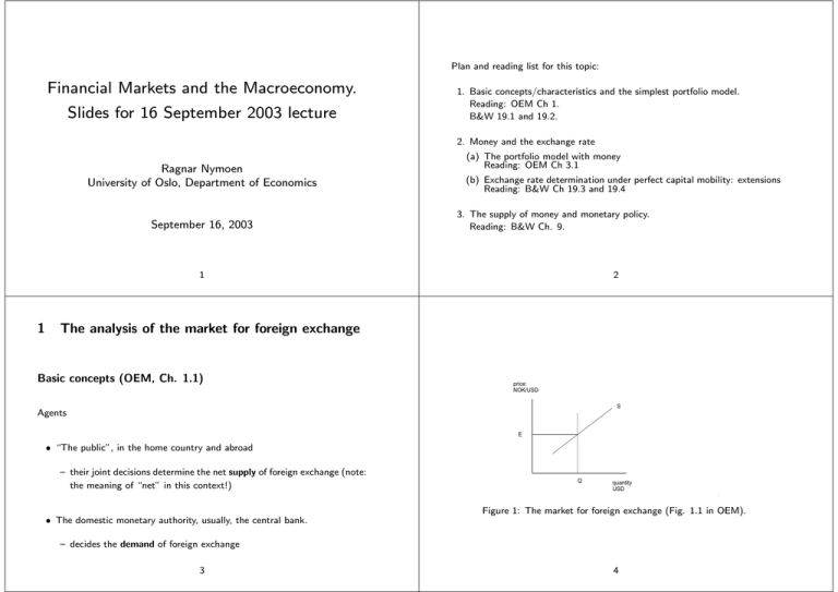
Plan and reading list for this topic:
Financial Markets and the Macroeconomy.
Slides for 16 September 2003 lecture
1. Basic concepts/characteristics and the simplest portfolio model.
Reading: OEM Ch 1.
B&W 19.1 and 19.2.
2. Money and the exchange rate
Ragnar Nymoen
University of Oslo, Department of Economics
September 16, 2003
(a) The portfolio model with money
Reading: OEM Ch 3.1
(b) Exchange rate determination under perfect capital mobility: extensions
Reading: B&W Ch 19.3 and 19.4
3. The supply of money and monetary policy.
Reading: B&W Ch. 9.
2
1
1
The analysis of the market for foreign exchange
Basic concepts (OEM, Ch. 1.1)
price:
NOK/USD
S
Agents
E
• “The public”, in the home country and abroad
— their joint decisions determine the net supply of foreign exchange (note:
the meaning of “net” in this context!)
Q
quantity
USD
Figure 1: The market for foreign exchange (Fig. 1.1 in OEM).
• The domestic monetary authority, usually, the central bank.
— decides the demand of foreign exchange
3
4
In the graph we have drawn the (governments) demand for foreign currency
(here USD) as a vertical line. A synonym is the foreign exchange reserve and
it denoted Q in the graph.
Q is the whole stock of foreign currency deposited in the central bank, less any
debt (incurred by the government) in foreign currency.
The supply schedule is market “S” and is upward sloping, i.e., supply is increasing in price.
Note:demand and supply relate to the whole stock of foreign currency
What determines net supply of foreign currency?
• In the short-run, it cannot be the trade balance (primary current account),
which is a flow variable.
• instead factors that can, in any point in time, effect a revaluation of existing
assets.
Hence, in the short-run factors like GDP growth and inflation are of little importance compared to the factors that are capable of shifting the net demands
of stocks (the exchange rate, interest rates at home and abroad and expectations).
Thus, the market for foreign exchange has characteristics in common with other
asset markets (residential housing, stock markets, world market for some raw
materials). In the short-run, supply (or demand) is fixed, so a sudden shift in
“the other side of the market” will typically result in an immidiate price change.
Important difference from market for manufactures and labour!
In the long-run, in a hypothetical steady-state, the primary current account is
however of great importance, see separate section below (OEM ch 1.6), since
private and government savings will have to be allocated to foreign or domestic
assets
5
Return to Figure 1 to define the main regimes on the foreign exchange market:
Assume that the initial situation is where the two schedules intersect, A. Thus
the exchange rate E is equilibrium exchange rate. Assume that there is a
positive (horizontal) shift in the S-curve. The new equilibrium depends in the
exchange rate regime:
• A →B
6
2
The balance sheet (OEM, Ch 1.2)
3 sectors (“agents”), 2 types of assets: Kroner assets and USD assets.
• g = “government”, i.e., the domestic monetary authority (central government and the central bank),
Floating exchange rate.
• p = private domestic investors,
• A → C
Fixed exchange rate. The central bank intervenes in the
market and increases its demand for USD (the foreign exchange reserves
increases).
7
• ∗ = foreign investors.
8
Government
Kr-assets
Bg
USD-assets
Fg
Net assets (in kroner) Bg + EFg
Private
Bp
Fp
EFp + Bp
Foreign
B∗
F∗
B∗ + EF∗
P and P∗ denotes domestic and foreign price levels. After multiplication of W∗
EP∗
by
, foreign and domestic wealths cancel:
P
EP∗
Wg + Wp +
W∗ = 0
P
For reference, we write Fg as
Sum
0
0
0
Table 2: Net financial assets, by sector (Table 1.1)
Fg = −(Fp + F∗),
The two first rows give
Bg + Bp + B∗ = 0
(1.1)
Fg + Fp + F∗ = 0
(1.2)
We can also use the table to define the sectors’ real wealth:
B + EFi
Wi = i
, i = g, p
P
B∗ + F∗E
W∗ =
P∗E
stating that the net supply of foreign exchange is the negative of the net demand
of the two other sectors’ demand.
Next add a subscript “0” which indicates net assets at the start of the period.
If the period is short in calendar time, financial wealth is unchanged at the end
of the period:
Bi + EFi = Bi0 + EFi0, i = g, p, ∗
however Bi and Fi can change a lot in the period, through asset-trade. In a
floating exchange rate regime, this is what drives the short run fluctuations in
the exchange rate.
10
9
3
A simple portfolio model (OEM (1.3) and 1.4)
Bp0 + EFp0
P
B∗0/E + F∗0
W∗ =
P
r = i − i∗ − ee
Wp =
How do we define “short period”?. A period so short that net financial savings
has negligible influence on total wealth, see ch 1.6.
April 1992:
Trade in the market for foreign exchange :
Foreing trade with goods (exports + imports)
(1.5)
300 bill
30 bill
ee
EFp
P
F∗
P∗
Fg + Fp + F∗
(1.11)
(1.12)
(1.13)
= ee(E)
(1.14)
= f (r, Wp), fr < 0, 0 < fW < 1
(1.15)
= W∗ − b(r, W∗), 0 < bw < 1, br > 0
(1.16)
=0
(1.17)
(1.11), (1.12) and (1.17) are lifted from the balance sheet.
(1.12) defines the risk premium r (see Ch 1.3). i∗ denotes the foreign interest
11
12
rate and ee is the expected rate of depreciation
To define the supply function formally: Start with (1.17):
e
( dE
dt )
d ln E e
ee =
≈
E
dt
In (1.14), the expected rate of depreciation is a function of the exchange rate:
0
regressive expectations
0
extrapolative
0
constant
ee < 0
ee > 0
ee = 0
Fg = −(Fp + F∗),
and substitute Fp and F∗ with the expressions in the other equations of the
model. The result is equation (1.18) in the book, or in more general notation:
Fg = S(E, P, P∗, i, i∗, Bp0, Fp0, B∗0, F∗o)
Equation (1.15) and(1.16) are demand functions (for domestic and foreign
investors (see Ch. 1.3)).
Exercise 3.1 Differentiate (1.18) in the book and show that (subject to Fp =
Fp0 and B∗ = B∗0)
SE ≡
7 equations.
∂Fg
P 0
P
= 2 γ − κee
∂E
E
E
where
• Endogenous: Wp, W∗, r, ee, Fp, F∗ and Fg or E (depending on regime)
• Exogenous: P, P∗, i, i∗, Bp0, Fp0, B∗0, F∗o and Fg or E (depending on
regime)
Use this to show that a set of sufficient conditions for an increasing supply
curve is
Fp0 > 0, Bo∗ > 0,
0
fW < 1, bw < 1, ee < 0.
((1.21))
Exercise 3.2 What are the consequences of a downward sloping supply curve?
15
EFp0
B
+ (1 − bw ) ∗0
P
P
EP∗
κ = −fr +
br > 0
P
γ = (1 − fW )
14
13
(*)
(1.19)