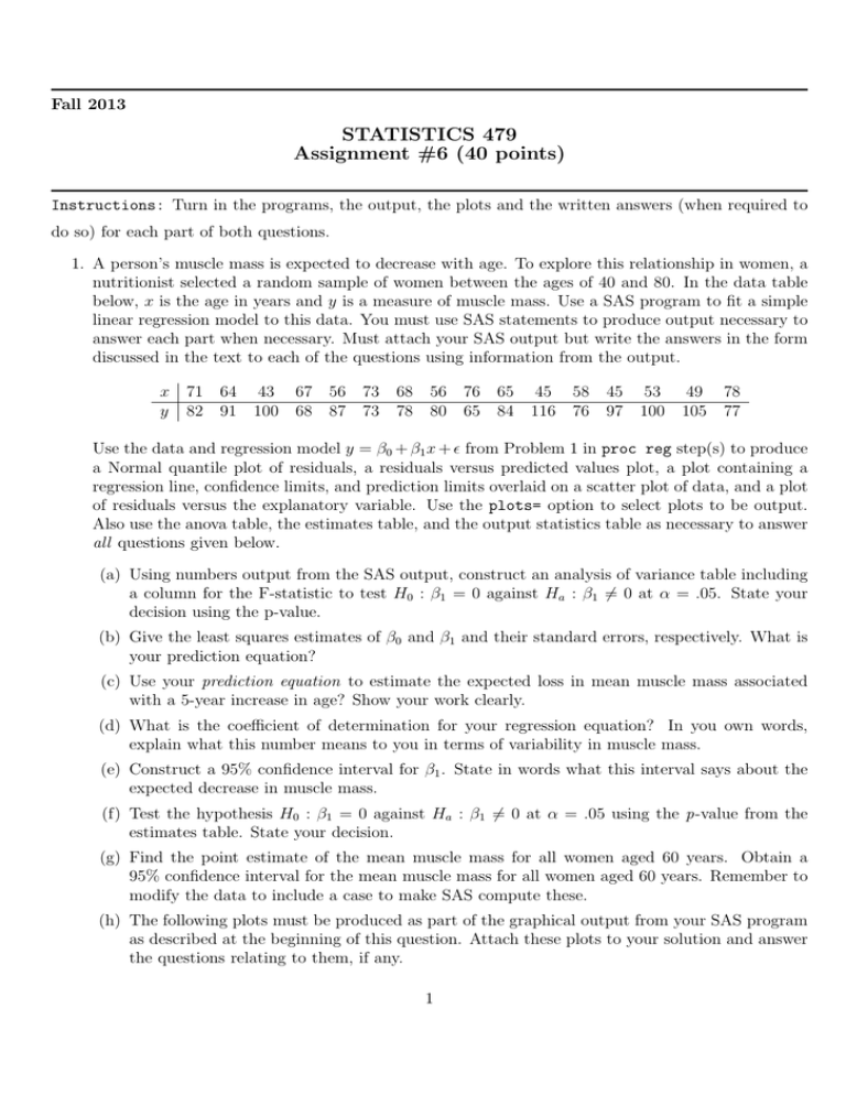
Fall 2013
STATISTICS 479
Assignment #6 (40 points)
Instructions: Turn in the programs, the output, the plots and the written answers (when required to
do so) for each part of both questions.
1. A person’s muscle mass is expected to decrease with age. To explore this relationship in women, a
nutritionist selected a random sample of women between the ages of 40 and 80. In the data table
below, x is the age in years and y is a measure of muscle mass. Use a SAS program to fit a simple
linear regression model to this data. You must use SAS statements to produce output necessary to
answer each part when necessary. Must attach your SAS output but write the answers in the form
discussed in the text to each of the questions using information from the output.
x 71
y 82
64
91
43 67 56 73 68 56 76 65
100 68 87 73 78 80 65 84
45
116
58 45 53
76 97 100
49
105
78
77
Use the data and regression model y = β0 + β1 x + from Problem 1 in proc reg step(s) to produce
a Normal quantile plot of residuals, a residuals versus predicted values plot, a plot containing a
regression line, confidence limits, and prediction limits overlaid on a scatter plot of data, and a plot
of residuals versus the explanatory variable. Use the plots= option to select plots to be output.
Also use the anova table, the estimates table, and the output statistics table as necessary to answer
all questions given below.
(a) Using numbers output from the SAS output, construct an analysis of variance table including
a column for the F-statistic to test H0 : β1 = 0 against Ha : β1 6= 0 at α = .05. State your
decision using the p-value.
(b) Give the least squares estimates of β0 and β1 and their standard errors, respectively. What is
your prediction equation?
(c) Use your prediction equation to estimate the expected loss in mean muscle mass associated
with a 5-year increase in age? Show your work clearly.
(d) What is the coefficient of determination for your regression equation? In you own words,
explain what this number means to you in terms of variability in muscle mass.
(e) Construct a 95% confidence interval for β1 . State in words what this interval says about the
expected decrease in muscle mass.
(f) Test the hypothesis H0 : β1 = 0 against Ha : β1 6= 0 at α = .05 using the p-value from the
estimates table. State your decision.
(g) Find the point estimate of the mean muscle mass for all women aged 60 years. Obtain a
95% confidence interval for the mean muscle mass for all women aged 60 years. Remember to
modify the data to include a case to make SAS compute these.
(h) The following plots must be produced as part of the graphical output from your SAS program
as described at the beginning of this question. Attach these plots to your solution and answer
the questions relating to them, if any.
1
i. Obtain a graph with plots of the 95% confidence interval and 95% prediction interval
curves for the fitted regression line overlaid on a scatter plot of the original data.
ii. Obtain a scatter plot of residuals against the x variable. Does this plot to explain whether
the straight line model is adequate or not? Explain.
iii. Obtain a normal probability plot residuals and a plot of residuals against the predicted values variable. Do these plots indicate that any of the model assumptions are not plausible?
In particular, is the assumption of normal errors reasonable? Explain.
2. It is reasonable to expect that heavier an automobile is it will be less efficient as reflected by the
miles per gallon (MPG) rating of the vehicle. The following data give MPG ratings (y) under city
driving conditions and the weight (x) of a random sample of 16 new vehicles.
Automobile Weight(lbs.)
ID
x
A
2620
B
2875
C
2320
D
3215
E
3440
F
3510
G
3570
H
2790
I
3150
J
3240
K
3670
L
3730
M
2200
N
2465
O
1835
P
2045
MPG
y
16.0
21.0
22.8
21.4
18.7
19.1
14.3
24.4
22.8
19.2
16.4
17.3
30.4
25.5
31.9
26.3
Use a SAS program to fit a single variable regression model and obtain all residual case statistics
and diagnostic plots discussed in class. Also use proc sgplot to obtain a scatterplot of the data with
each point labeled using the Vehicle Id.
(a) Are there any cases that are x-outliers? Explain.
(b) Are there any cases that are y-outliers? Explain.
(c) The Cook’s D statistic for some of these cases are ’large’. Explain reasons for this by using
the fact Cook’s D is a product of functions of studentized residuals and hat diagonals.
(d) Suppose that the model is refitted after the vehicles labeled A and O are deleted from the data
set one at a time. Discuss the model fit for each of these compared with the fit of the original
model.
(e) Explain the effect of these cases on the model fit by using the appropriate case statistics output
from the model fit to the original data.
Due Thursday, November 7, 2013
2