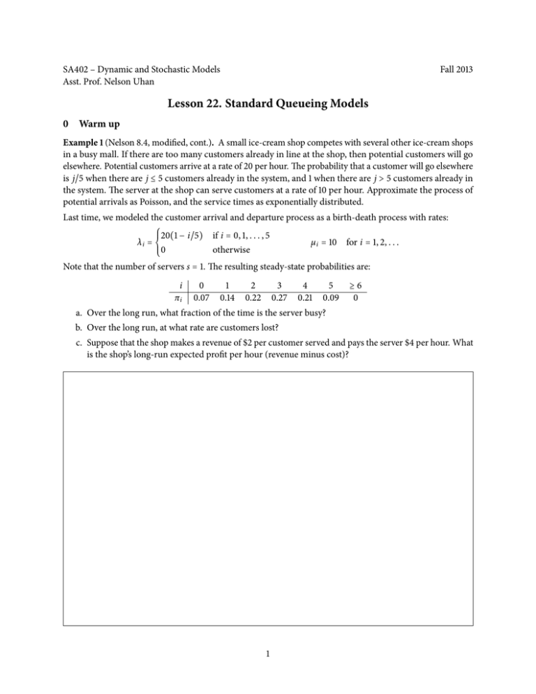
SA402 – Dynamic and Stochastic Models
Asst. Prof. Nelson Uhan
Fall 2013
Lesson 22. Standard Queueing Models
0
Warm up
Example 1 (Nelson 8.4, modified, cont.). A small ice-cream shop competes with several other ice-cream shops
in a busy mall. If there are too many customers already in line at the shop, then potential customers will go
elsewhere. Potential customers arrive at a rate of 20 per hour. The probability that a customer will go elsewhere
is j/5 when there are j ≤ 5 customers already in the system, and 1 when there are j > 5 customers already in
the system. The server at the shop can serve customers at a rate of 10 per hour. Approximate the process of
potential arrivals as Poisson, and the service times as exponentially distributed.
Last time, we modeled the customer arrival and departure process as a birth-death process with rates:
⎧
⎪
⎪20(1 − i/5) if i = 0, 1, . . . , 5
µ i = 10 for i = 1, 2, . . .
λi = ⎨
⎪
0
otherwise
⎪
⎩
Note that the number of servers s = 1. The resulting steady-state probabilities are:
i
πi
0
0.07
1
0.14
2
0.22
3
0.27
4
0.21
5
0.09
≥6
0
a. Over the long run, what fraction of the time is the server busy?
b. Over the long run, at what rate are customers lost?
c. Suppose that the shop makes a revenue of $2 per customer served and pays the server $4 per hour. What
is the shop’s long-run expected profit per hour (revenue minus cost)?
1
1
Standard queueing notation
● Standard notation for queues:
arrival process / service process / s / n / k / queue discipline
● Arrival process (interarrival times usually assumed to be independent and time stationary)
○ M = Markovian (Poisson process / exponential interarrival times)
○ G = General distribution
○ D = deterministic (fixed interarrival times)
○ Ek = Erlang with k phases
● Service process (service times usually assumed to be independent and time stationary)
○ M = Markovian (exponential service time)
○ D = deterministic (fixed service times)
○ G, Ek
● s = number of servers
● n = system capacity (e.g. number of customers that can be in the shop)
● k = number of potential customers (size of customer population)
● Queueing discipline:
○ FIFO = first in first out (equivalently, FCFS = first come first served)
○ LIFO = last in first out (equivalently, LIFO = last come first served)
○ SIRO = service in random order
● If not specified, default values:
○ n=∞
○ k=∞
○ queueing discipline = FIFO
● Two fundamental standard queues:
○ M/M/∞: birth-death process with
○ M/M/s: birth-death process with
2
2 The M/M/∞ queue
● Let’s apply the formulas for the steady-state probabilities:
πj =
dj
∑∞
i=0 d i
j
for j = 0, 1, 2, . . .
where
d0 = 1,
dj = ∏
i=1
λ i−1
µi
for j = 1, 2, . . .
● We can simplify d j :
● Therefore, we can rewrite ∑∞
j=0 d j :
● As a result, the steady-state probabilities for a M/M/∞ queue are:
● The number of customers in steady state L is
Example 2. Recall the Massive Mall case: we want to determine the number of parking spaces needed for
the new mall by pretending that parking is unlimited, and then investigating how many spaces are sufficient
to satisfy demand a large fraction of the time. Assume customers arrive according to a Poisson process with
arrival rate λ = 1000 per hour. In addition, suppose the time that a customer spends at the mall is exponentially
distributed with rate µ = 1/3.
a. What is the expected number of cars in the parking lot?
b. What is the expected time a car spends in the parking lot?
c. What is the minimum number of parking spaces needed to hold all cars 99.9% of the time?
3
3 The M/M/s queue
● Steady-state probabilities: using ρ = λ/(sµ),
⎧
(λ/µ) j
⎪
⎪
⎪
π0
⎪
⎪
π j = ⎨ j! j
⎪
(λ/µ)
⎪
⎪
⎪
π
⎪
⎩ s!s j−s 0
⎡ s
⎤−1
⎢
(sρ) j
s s ρ s+1 ⎥⎥
⎢
π 0 = ⎢( ∑
)+
s!(1 − ρ) ⎥⎥
⎢ j=0 j!
⎣
⎦
for j = 1, 2, . . . , s
for j = s + 1, s + 2, . . .
● Expected number of customers in queue and expected delay:
ℓq =
πs ρ
(1 − ρ)2
wq =
ℓq
πs ρ
=
λ λ(1 − ρ)2
● Expected number of customers in the system and expected waiting time:
ℓ = λw = ℓ q +
λ
µ
w = wq +
1
µ
Example 3. Recall the Darker Image case: we considered adding a second photocopier to the copy shop.
Suppose customers arrive according to a Poisson process with rate 4 customers per hour, and that the service
time of each photocopier is exponentially distributed with a mean of 12 minutes. Compare the expected delay
of customers when there is 1 copier vs. when there are 2 copiers.
4
4
The G/G/s queue
● When interarrival times and service times are not Markovian (exponentially distributed), things get
much harder
● We can still use results from Markovian queues to approximate performance measures, usually with a
“correction”
● Setup:
○ G = generic interarrival time random variable with λ = 1/E[G]
○ X = generic service time random variable with µ = 1/E[X]
○ Squared coefficients of variation:
εa =
Var[G]
E[G]2
εs =
Var[X]
E[X]2
● Let ŵ q be the expected delay in this G/G/s queue
● Let w q be the expected delay in a M/M/s queue with arrival rate λ and service rate µ
● Whitt’s (1983) approximation:
ŵ q ≈
ε a + εs
wq
2
● We can use this with Little’s law (both versions) to find approximations of ℓ q , ℓ, and w
● This approximation works well when ρ, ε a , and εs are “close” to 1
● When G ∼ Exp(λ) and X ∼ Exp(µ): Var(G) =
⇒ εa =
, εs =
, Var(X) =
⇒
● Note: Whitt’s (1983) is one of many approximations that have been proposed for G/G/s queues
Example 4. Consider the Darker Image case again. Suppose now that the service time of each photocopier is
uniformly distributed between 2 and 8 minutes. Now compare the expected delay of customers when there is 1
copier vs. when there are 2 copiers.
5