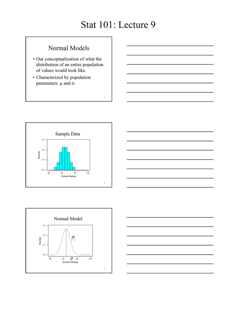
Stat 101: Lecture 9
Normal Models
• Our conceptualization of what the
distribution of an entire population
of values would look like.
• Characterized by population
parameters: μ and σ.
1
Sample Data
0.3
Density
0.2
0.1
0.0
85
90
95
100
Octane Rating
2
Normal Model
0.3
σ
Density
0.2
0.1
0.0
85
90
μ
95
100
Octane Rating
3
Stat 101: Lecture 9
Normal Model
• Octane Rating
• Center:
– Mean, μ = 91
• Spread:
– Standard deviation, σ=1.5
4
68-95-99.7 Rule
• 68% of the values fall within 1
standard deviation of the mean.
• 95% of the values fall within 2
standard deviations of the mean.
• 99.7% of the values fall within 3
standard deviations of the mean.
5
Octane Rating
• 68% of the values fall between
89.5 and 92.5.
• 95% of the values fall between
88.0 and 94.0.
• 99.7% of the values fall between
86.5 and 95.5.
6
Stat 101: Lecture 9
Normal Percentiles
• What percentage of octane ratings
fall below 92?
• Draw a picture.
• How far away from the mean is 92
in terms of number of standard
deviations?
7
0.3
Density
0.2
Shaded
Area
0.1
0.0
90
85
92
95
100
Octane Rating
8
Standard Normal Model
z=
92 − 91
= 0.67
1.5
• Table Z: in your text.
• http://davidmlane.com/hyperstat/z_tab
le.html
9
Stat 101: Lecture 9
From Percentiles to Scores
• What octane rating corresponds to
the 25th percentile?
• Draw a picture.
• The 25th percentile is how many
standard deviations away from the
mean?
10
0.3
Density
0.2
25%
0.1
0.0
85
90
95
100
Octane Rating
11
Standard Normal Model
• Table Z: in your text.
− 0.67 =
?− 91
1.5
• http://davidmlane.com/hyperstat/z_tab
le.html
12
Stat 101: Lecture 9
Are Your Data Normal?
• The histogram should be mounded
in the middle and symmetric.
• The data plotted on a normal
probability (quantile) plot should
follow a diagonal line.
3
.99
2
.95
.90
1
.75
0
.50
.25
Normal Quantile Plot
13
-1
.10
.05
-2
.01
-3
6
4
Count
8
2
90
Octane Rating
95
14
3
.99
2
.95
.90
.75
.50
1
0
.25
.10
.05
.01
Normal Quantile Plot
85
-1
-2
-3
25
15
Count
20
10
5
7.5
8
8.5
9
9.5
10 10.5 11 11.5 12
Amplifier Gain (dB)
15