advertisement
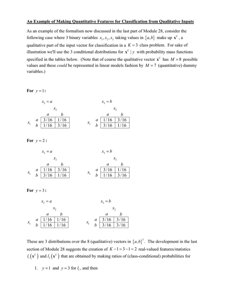
An Example of Making Quantitative Features for Classification from Qualitative Inputs As an example of the formalism now discussed in the last part of Module 28, consider the following case where 3 binary variables x1 , x2 , x3 taking values in a, b make up xC , a qualitative part of the input vector for classification in a K 3 class problem. For sake of illustration we'll use the 3 conditional distributions for x C | y with probability mass functions specified in the tables below. (Note that of course the qualitative vector xC has M 8 possible values and these could be represented in linear models fashion by M 7 (quantitative) dummy variables.) For y 1 : x3 a x3 b x2 x1 a b a 3 /16 1/16 x2 b 1/16 3 /16 x1 a b a 1/16 3 /16 b 3 /16 1/16 For y 2 : x3 a x3 b x2 x1 a b a 1/16 3 /16 x2 b 3 /16 1/16 x1 a b a 3 /16 1/16 b 1/16 3 /16 For y 3 : x3 a x3 b x2 x1 a b a 1/16 1/16 x2 b 1/16 1/16 x1 a b a 3 /16 3 /16 b 3 /16 3 /16 These are 3 distributions over the 8 (qualitative) vectors in a, b . The development in the last 3 section of Module 28 suggests the creation of K 1 3 1 2 real-valued features/statistics l1 x C and l2 x C that are obtained by making ratios of (class-conditional) probabilities for 1. y 1 and y 3 for l1 , and then 2. y 2 and y 3 for l2 . Values for these two features/statistics are given below in two forms. First, in two tables made by dividing values in corresponding cells of pairs of tables above we have: Values of l1 : x3 a x3 b x2 x1 a b a 3 1 x2 b 1 3 x1 a b a 1/ 3 1 b 1 1/ 3 Values of l2 : x3 a x3 b x2 x1 a b a 1 3 x2 b 3 1 x1 a b a 1 1/ 3 b 1/ 3 1 Then, in a single table listing all 8 values of x C and then l1 x C and l2 x C and their logarithms, we have: xC a, a, a b, a, a a, b, a b, b, a a, a, b b, a, b a, b, b b, b, b l1 x C l2 x C ln l1 x C ln l2 x C 3 1 1.099 0 1 3 0 1.099 1 3 0 1.099 3 1 1.099 0 1/ 3 1 1.099 0 1 1/ 3 0 1.099 1 1/ 3 0 1.099 1/ 3 1 1.099 0
