here - James Hall Business Solutions
www.james-hall.com
Vlookups are really easy...
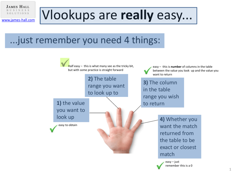
...just remember you need 4 things:
Half easy – this is what many see as the tricky bit, but with some practice is straight forward
2) The table range you want to look up to
1) the value you want to look up easy to obtain easy – this is number of columns in the table between the value you look up and the value you want to return
3) The column in the table range you wish to return
4) Whether you want the match returned from the table to be exact or closest match easy – just remember this is a 0
1
www.james-hall.com
An example
We have been given a list of part numbers from Purchasing, (see green cells) and want to look to up against a list given to us from Engineering (see blue cells) and return the quantity for each green celled part number in column A when matched against the equivalent part number in column D and the corresponding quantity retrieved from column F a) Click in cell B2, this is where we want to start the formula b) Click the ‘fx’ symbol and from the menu choose ‘All’
(scroll to 13 th function from end ‘vlookup’) c) From the menu that appears fill it out as follows
(screenshot bottom right below) d) Finally click on OK
Click on column D row header and drag it to column E
Starting at column D count to the right the column the quantity is in (D=1, E=2,
F=3, so in this case 3) b) c) a)Click in cell B2
Is always 0, type in 0 d)
2
www.james-hall.com
Example cont.
The answer 60 will appear in cell B2. Click in Cell B2 and then put the mouse pointer on the bottom right hand corner of the cell so it changes to a cross hair. Click the left mouse button when the cross hair is selected and then copy this down to cell B7. The
Quantity values will then appear for the other part numbers
3
www.james-hall.com
Summary - Speaking Excel’s Language
To understand how a vlookup works we have to think like Excel and talk its language.
As humans we say “we want to look at this value in this part of the spreadsheet against this list and return me back this column making sure its an exact match”
For Excel to perform a vlookup we need to express out instructions in the following formula, it looks complex but its just how we instruct Excel :
=
=vlookup( A2, D:F, 3, 0)
2) The table range you want to look up to
(table bound by column D:F)
3) The column in the table range you wish to return (D to F) =3
4) easy – just remember this is always a 0
On our screens it will look as follows:
=vlookup(A2,D:F,3,0)
1) the value you want to look up, e.g. its in cell A2
4
www.james-hall.com
If it will still not work…
…then the solution will be in here:
1) If you have two totally separate sessions of Excel running then Excel will not perform the vlookup as it cannot make the ‘link’ between the lists (solution, save all your files, close all sessions of Excel, re-open one Excel program and open your files in the one ‘session’ of Excel and perform the vlookup again)
2) You have numbers stored as text looking up against numbers stored as numbers in your other list (or visa versa) so the vlookup will not work. Solution – make sure you are looking up numbers stored as text to another list of numbers stored as text or numbers stored as numbers to another list of numbers
stored as numbers – if you mix the two the vlookup will not work. To turn a number stored as text into a
number stored as number we can use for calculation =value(A1). Convert all your numbers stored as text to real numbers and perform your vlookup again. If for some reason you want to turn a number back to text after then use the command =text(A1,0)
3) One of your lists has a blank space (or number of blank spaces after it). Sometimes when we use data provided from computer generated report there can be blank spaces after the value finishes if it is text.
For example “James” will look like “James ” when stored in a cell, but the second instance of “James ” actually contains a space after the s. Check your lists for hidden spaces – if they are there then delete them and re perform the vlookup. To do this automatically use the formula =TRIM(A2)
5
