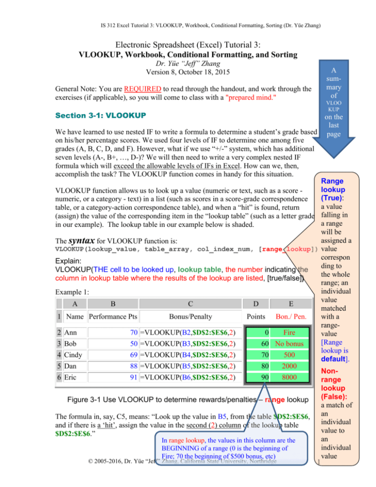
IS 312 Excel Tutorial 3: VLOOKUP, Workbook, Conditional Formatting, Sorting (Dr. Yüe Zhang)
Electronic Spreadsheet (Excel) Tutorial 3:
VLOOKUP, Workbook, Conditional Formatting, and Sorting
Dr. Yüe “Jeff” Zhang
Version 8, October 18, 2015
General Note: You are REQUIRED to read through the handout, and work through the
exercises (if applicable), so you will come to class with a "prepared mind."
Section 3-1: VLOOKUP
We have learned to use nested IF to write a formula to determine a student’s grade based
on his/her percentage scores. We used four levels of IF to determine one among five
grades (A, B, C, D, and F). However, what if we use “+/-” system, which has additional
seven levels (A-, B+, …, D-)? We will then need to write a very complex nested IF
formula which will exceed the allowable levels of IFs in Excel. How can we, then,
accomplish the task? The VLOOKUP function comes in handy for this situation.
A
summary
of
VLOO
KUP
on the
last
page
Range
lookup
VLOOKUP function allows us to look up a value (numeric or text, such as a score (True):
numeric, or a category - text) in a list (such as scores in a score-grade correspondence
a value
table, or a category-action correspondence table), and when a “hit” is found, return
(assign) the value of the corresponding item in the “lookup table” (such as a letter grade falling in
a range
in our example). The lookup table in our example below is shaded.
will be
assigned a
The syntax for VLOOKUP function is:
VLOOKUP(lookup_value, table_array, col_index_num, [range_lookup]) value
correspon
Explain:
ding to
VLOOKUP(THE cell to be looked up, lookup table, the number indicating the
the whole
column in lookup table where the results of the lookup are listed, [true/false])
range; an
individual
Example 1:
value
A
B
C
D
E
matched
1 Name Performance Pts
Bonus/Penalty
Points Bon./ Pen.
with a
range2 Ann
70 =VLOOKUP(B2,$D$2:$E$6,2)
0
Fire
value
[Range
3 Bob
50 =VLOOKUP(B3,$D$2:$E$6,2)
60 No bonus
lookup is
4 Cindy
69 =VLOOKUP(B4,$D$2:$E$6,2)
70
500
default].
5 Dan
88 =VLOOKUP(B5,$D$2:$E$6,2)
80
2000
Non6 Eric
91 =VLOOKUP(B6,$D$2:$E$6,2)
90
8000
range
lookup
(False):
Figure 3-1 Use VLOOKUP to determine rewards/penalties – range lookup
a match of
an
The formula in, say, C5, means: “Look up the value in B5, from the table $D$2:$E$6,
individual
and if there is a ‘hit’, assign the value in the second (2) column of the lookup table
value to
$D$2:$E$6.”
an
In range lookup, the values in this column are the
individual
BEGINNING of a range (0 is the beginning of
Fire; 70 the beginning of $500 bonus, etc)
value
© 2005-2016, Dr. Yüe “Jeff” Zhang, California State University, Northridge
1
IS 312 Excel Tutorial 3: VLOOKUP, Workbook, Conditional Formatting, Sorting (Dr. Yüe Zhang)
What does the last argument “True/False” mean? --=VLOOKUP(B2,$D$2:$E$6,2, True) ---- (1)
Or
=VLOOKUP(B2,$D$2:$E$6,2, False) ---- (2)
(1) is default (if you don’t enter anything for this argument), and (2) has to be explicitly
specify. The difference? Situation (1) requires the first column of the lookup table to be
in ascending order, while (2) does not, i.e, the first column can be in any order.
Example 2:
A
B
C
1 Name TransactionID
D
Transaction/Charge
E
TransID Charge
2 Ann
1070 =VLOOKUP(B2,$D$2:$E$6,2, False)
1391 $1,020
3 Bob
2050 =VLOOKUP(B3,$D$2:$E$6,2, False)
2050 $1,100
4 Cindy
1169 =VLOOKUP(B4,$D$2:$E$6,2, False)
2288 $3,220
5 Dan
2288 =VLOOKUP(B5,$D$2:$E$6,2, False)
1169 $2,120
6 Eric
1391 =VLOOKUP(B6,$D$2:$E$6,2, False)
1070 $520
Figure 3-1 Use VLOOKUP to determine charges for transactions – non-range lookup
1
2
3
4
VLOOKUP(Val_to_look, Table, Column_to_retun, Range_or_not)
If the last argument (4 above) is default (True),
the first column must be ascending – in that case
it’s a range lookup, MEANING: the number/text
to be looked up would fall into a certain range
the whole of which correspond to one value in
the returned value column;
If the last argument (4 above) is False, the first
column can be in any sequence – in that case it’s
a non-range lookup, MEANING: the number/text
to be lookup should EXACTLY match a certain
value in the lookup column which will return one
value from the returned value column;
The returned value column can be anything (text,
number, mix of the two)
If there’s such
correspondence:
11-20  A
21-30  B
What would 25
correspond to?
If there’s such
correspondence:
11 A, 21 B,
31 C,
What would 25
correspond to?
Say: scores 700-750 is V
Good; Sales over $10,000
has commission rate 2.5%
The returned value column can be the second,
third, … column in the lookup table (so the third
term in the VLOOKUP function would be…?)
© 2005-2016, Dr. Yüe “Jeff” Zhang, California State University, Northridge
2
IS 312 Excel Tutorial 3: VLOOKUP, Workbook, Conditional Formatting, Sorting (Dr. Yüe Zhang)
Explore: HLOOKUP function (horizontal lookup) works in a similar
fashion. You can try it yourself. The following is a section of a spreadsheet
showing HLOOKUP:
Row 1
Row 2
Section 3-2: Workbook – Referencing across Worksheets
1. A workbook contains multiple worksheets.
2. Worksheets are identified with their names shown in the worksheet tabs. The name of
a worksheet can be renamed in the same way as you rename a file.
3. When you need to refer to a cell in ANOTHER worksheet, use the format in the
following example (assuming you want to calculate total cost):
Total Cost = Fixed cost + Volume * Variable Cost
If each of the values is in the same cell address on different sheet, say
B1 on sheet "FixedCost" stores fixed cost,
B1 on sheet "Volume" stores volume,
B1 on sheet "VariableCost" stores variable cost,
B1 on sheet "TotalCost" is the formula that you are creating to calculate total cost, then
you have in sheet "TotalCost", cell B1 the following formula:
=FixedCost!B1+Volume!B1*VariableCost!B1
where the "!" means "sheet".
You can do sum or average across sheets in a similar fashion, for example:
=average(sheet1!g3, sheet2!g3, sheet3!g3) or =average(sheet1:sheet3!g3)
Section 3-3: Conditional Formatting
XYZ Company recently had some customer complaints on the quality of some products
they produced. XYZ Company believes that their production processes are in normal
performance; but to be sure, they want you to run some statistical analyses to verify that.
Assume that you decide to run a t-test to determine whether the quality indicators of a
wide range of products are significantly different between Q1 and Q2. You can use the
feature of conditional formatting in Excel (and all other electronic spreadsheets) to find
those values less than the specified p value. Steps to perform conditional formatting:
© 2005-2016, Dr. Yüe “Jeff” Zhang, California State University, Northridge
3
IS 312 Excel Tutorial 3: VLOOKUP, Workbook, Conditional Formatting, Sorting (Dr. Yüe Zhang)
1. Highlight the cell
range that you want to
format;
2. On the ribbon,
select Home ribbon,
Styles group, then
Conditional
Formatting.
3. You can then select
from the drop-down
list the logical
relationship you need.
Here you want to
select less than.
1. Then you want to fill out the value(s) in the slot(s). Here you only have one value,
which is 0.05. Fill it in the first slot. (What if you want to set the condition
“between 0.05 and 0.1”? Think and try)
2. Click the Format button, and you will see a Format Cells dialog box pop up. You
can then choose the format you want, such as red color. Click OK, and see this:
Section 3-4: Sorting a Spreadsheet
IntelliImage, a company selling digital camera, digital camcorder (DV), and scanners, has
four sales regions - Las Vegas, Los Angeles, Phoenix, and San Francisco. The following
table shows the digital camera and DV sales of IntelliImage in the four sales regions.
© 2005-2016, Dr. Yüe “Jeff” Zhang, California State University, Northridge
4
IS 312 Excel Tutorial 3: VLOOKUP, Workbook, Conditional Formatting, Sorting (Dr. Yüe Zhang)
A
4
Sales ($million)
5
6
7
8
9
Las Vegas
Los Angeles
Phoenix
San Francisco
Product totals
B
Digital
Camera
20
14
8
18
60
C
DV
9
11
3
7
30
D
City
Totals
29
25
11
25
90
The VP for Marketing of IntelliImage would like to see the sales regions listed according
to their sales performance, highest first (descending). Here is what you would do:
(1) Highlight A4:D8 – data, city totals, and the column headers, but NOT “Product
totals”: you want to leave the product totals as the last row.
(2) Select Data on menu bar, select Sort, and a sort dialog box will appear as in the
figure below.
(3) You want to sort by City Totals. Click at the down-arrow button at the sort by box
and a drop-down list of fields would allow you to choose City Totals you want to sort
on.
(4) If you want to sort on a different field when there are more than one row having the
same city total, you can then choose a field in the Then by box. This would be your
secondary sorting field.
Sort by City Total
(5) Click OK and your data is sorted!
(6) Similarly, you can sort on other fields such as Digital Camera or DV.
© 2005-2016, Dr. Yüe “Jeff” Zhang, California State University, Northridge
5
IS 312 Excel Tutorial 3: VLOOKUP, Workbook, Conditional Formatting, Sorting (Dr. Yüe Zhang)
SUMMARY on VLOOKUP
VLOOKU
P
VLOOKU
P
(Item 1,
VLOOKUP Syntax:
Item 2,
(Value to look up
Lookup table
T (or 1) Range Lookup
Item 3,
Item 4)
Column # (in
the table) to get
the value
Range lookup
– True/False)
Can be
omitted, in
which case
it’s the
default
value –
True (range
lookup)
F ( or 0) Non-Range
Lookup
Item #4
Omitted (default Must be
= True)
explicitly
indicated: False
1stcolumn
in lookup
table
How it
works
MUST be
ascending
Can be any
order
The value falls in
a given range in
the lookup table
falling in range
The value has an
exact match in
the lookup table
exact match
return the
value of
the indicated
column in
item #3
Interpretation
Match of a value to
its “range match” – if
you are between
range_begin and
range_end (like 70
and 79), you all get
the same match (like
grade C)
Match of a value to a
value – if you are a
specific a, you would
be matched with a
specific x; if a
specific b, matched
with specific y; etc.
Examples
- scores to grade;
- credit scores to
credit rating;
- ages to age group;
-taxable incomes to
tax bracket
- points earned to
membership class
-…
- name to address;
- state to capital;
- year to award
movie;
- transaction
number to charge
- stud ID to stud
DOB
-…
“Hit”
and
result
Think about these
scenarios; you may
see them in
exam/project.
© 2005-2016, Dr. Yüe “Jeff” Zhang, California State University, Northridge
6