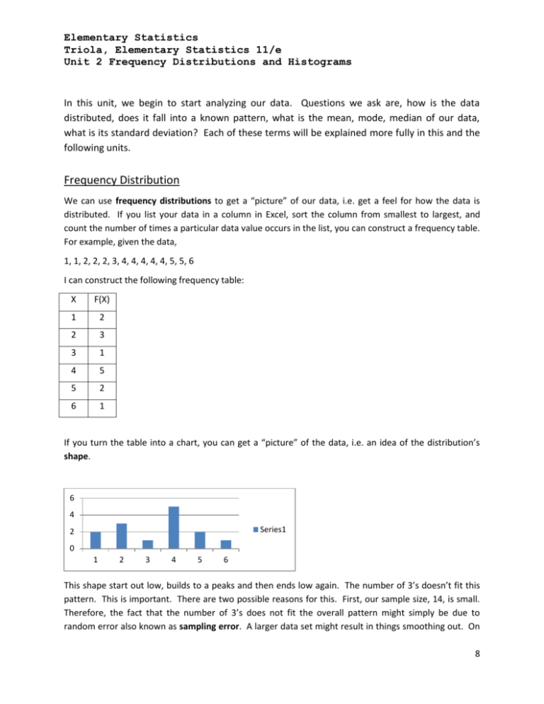
Elementary Statistics
Triola, Elementary Statistics 11/e
Unit 2 Frequency Distributions and Histograms
In this unit, we begin to start analyzing our data. Questions we ask are, how is the data
distributed, does it fall into a known pattern, what is the mean, mode, median of our data,
what is its standard deviation? Each of these terms will be explained more fully in this and the
following units.
Frequency Distribution
We can use frequency distributions to get a “picture” of our data, i.e. get a feel for how the data is
distributed. If you list your data in a column in Excel, sort the column from smallest to largest, and
count the number of times a particular data value occurs in the list, you can construct a frequency table.
For example, given the data,
1, 1, 2, 2, 2, 3, 4, 4, 4, 4, 4, 5, 5, 6
I can construct the following frequency table:
X
F(X)
1
2
2
3
3
1
4
5
5
2
6
1
If you turn the table into a chart, you can get a “picture” of the data, i.e. an idea of the distribution’s
shape.
6
4
Series1
2
0
1
2
3
4
5
6
This shape start out low, builds to a peaks and then ends low again. The number of 3’s doesn’t fit this
pattern. This is important. There are two possible reasons for this. First, our sample size, 14, is small.
Therefore, the fact that the number of 3’s does not fit the overall pattern might simply be due to
random error also known as sampling error. A larger data set might result in things smoothing out. On
8
Elementary Statistics
Triola, Elementary Statistics 11/e
Unit 2 Frequency Distributions and Histograms
the other hand, the population might actually be bimodal, in which case the two separate peaks, one a 2
and the other at 4 are significant. With such a small sample size, there isn’t any way to tell which is the
correct interpretation. The only thing we can do is to take a larger sample size. Remember this, it will
come up again.
A related concept is that of a relative frequency distribution. If you divide the results in the F(X) column
by the total number of data, you will get, essentially, percentages in decimal form.
X
F(X)
1
.14
2
.21
3
.07
4
.37
5
.14
6
.07
What would you guess that the number in F(X) column add up to? Write the answer on the Answer
Sheet for question #1.
Histograms
The chart shown on the previous page is called a histogram. Later, we will learn how to use Excel to
construct histograms, but for now it will suffice to see that a histogram is a chart of a frequency table.
Having one bar for each entry in the table works well for discrete data, but this falls apart when working
with continuous data. With continuous data, you are unlikely to get two data items with the same
value. In this case, you have to construct what we call bins, which basically are data intervals. For
example, open up the data set, Washer I.D. Data and look at Sheet 2. This sheet shows the bins used for
the histogram of the data in column A.
Technical Note:
In Excel, the bin value is the upper end of the interval.
For example, the second bin in the worksheet, 24.75 captures all data falling
in the range, 𝟐𝟒. 𝟕𝟎 < 𝐱 ≤ 𝟐𝟒. 𝟕𝟓. The first bin, 24.7 captures all data 24.7 and less.
Selecting the best number of bins is somewhat science and somewhat art. You don’t want too many
bins, because then you distribution will be too “thin”, i.e. not enough data in each bin. You also don’t
what too few bins because then the distribution will be too “fat”, i.e. too much data going into each bin.
In these cases you don’t get a good idea of the shape of the distribution. The number of bins is up to
you, so you’ll probably want to play around a little until you get a good “picture” of your data.
9
Elementary Statistics
Triola, Elementary Statistics 11/e
Unit 2 Frequency Distributions and Histograms
There are two rules that have to be followed. First, each bin must be of the same width, and second,
you need to capture all of the data, so your bins need to cover the full range of the data. The width of a
bin can be calculated as follows:
𝑊𝑖𝑑𝑡ℎ =
𝐻𝑖𝑔ℎ𝑒𝑠𝑡 𝑉𝑎𝑙𝑢𝑒 − 𝐿𝑜𝑤𝑒𝑠𝑡 𝑉𝑎𝑙𝑢𝑒
𝑁𝑢𝑚𝑏𝑒𝑟 𝑜𝑓 𝐷𝑒𝑠𝑖𝑟𝑒𝑑 𝐵𝑖𝑛𝑠
Look at sheet 2 of the Excel spreadsheet Washer I.D. Data. There you will see the bins chosen, the
frequency table and a chart based on the table. Would you consider the distribution to be roughly
symmetrical, i.e. the left side is almost a mirror image of the right side, with the axis of symmetry being
around 20.05? Write your answer on the Answer Sheet for question #2.
Does it start out low, build to a peak and then drop off? Answer for question #3 on the Answer Sheet.
A distribution with this kind of shape is said to be Normally distributed. Normal distributions will be
very important to us in our study of statistics.
Now, try your hand at creating a histogram. First read the pages on How to Use Excel to Histogram
which you will find in the appendix to the workbook (For now, you’ll find it on the website,
ronharrow.com, under Statistics->Miscellaneous). Now open the data set, Lab Mice Data, select Sheet
2, and using the bins provided, create your own histogram of the data.
Print the histogram, put your name on it and bring it to class.
Percentiles
The percentile corresponding to a score is the percentage of the scores that fall below that score. For
example, if you have an IQ of 120 then you will be in the 91st percentile because 91% of the population
will have an IQ below yours.
Excel has two stat functions for working with percentiles, PERCENTILE.INC and PERCENTRANK.INC. See
the note on How to Work With the Stat Menu in Excel (under Statistics->Miscellaneous). Open up the
data set, Test Scores and use PERCENTILE.INC to find the score corresponding to the 75th percentile (use
0.75)
Write your answer on the Answer Sheet for question #4.
Now use the PERCENTILERANK.INC function to find the percentile corresponding to the score 88.5.
Answer for question #5.
There are two side topics worth mentioning here. The first is outliers. It’s not unusual to get a few data
values that just don’t fit in with the rest of the data. Sometimes it’s simply due to pilot error or sampling
10
Elementary Statistics
Triola, Elementary Statistics 11/e
Unit 2 Frequency Distributions and Histograms
error. Other times there might be a perfectly good explanation. For example, consider the following
launch times for the shuttle,
13.4, 14.3, 12.9, 14.1, 13.6, 0.0
Clearly, the 0.0 is an outlier. What’s the explanation? The shuttle simply failed to launch that time.
However, there may be outliers that have no explanation. For example, a puzzle that confounded
astronomers for a long time was that the orbit of Mercury appeared to wobble. Planetary orbits should
be perfectly elliptical. It turned out this this outlier was very important, and the observed orbit was due
to the relativistic effects of being so close the sun’s gravity well. Mercury’s strange orbit wasn’t
understood until Einstein came along.
So, how should you deal with outliers? Typically, you’ll leave them out of your analysis because under
many circumstances they can render the results useless. However you must carefully document their
existence as well as their explanation if possible.
Another interesting side topic is Pareto Analysis. Pareto was a nineteenth century Italian engineer. His
significant discovery was that 80% percent of a problem can be explained by 20% of all the possible
causes, the so called 80-20 rule. As an example of this rule, consider software bugs. There are many
kinds of software errors, and there are many causes, well over 100 identified causes. However, 80% of
all bugs can be traced to only 20% of all causes. This is a very powerful idea because it enables us mere
mortals to effectively attack problems. When we encounter a software bug, the first place we look at
are the 20 or so most common reasons, before we look at the other 80. 80% of the time we will find our
cause among the 20 quickly and effectively and get the software running again. Pareto analysis is used
heavily throughout the business and engineering world and everyone should be familiar with it.
This is the end of Unit 2.
Turn now to your MyMathLab homework to get more
practice with these concepts.
11
Elementary Statistics
Triola, Elementary Statistics 11/e
Unit 2 Frequency Distributions and Histograms
____________________________
Name
Answer Sheet
1. ______________
2. ______________
3. ______________
4. ______________
5. ______________
12