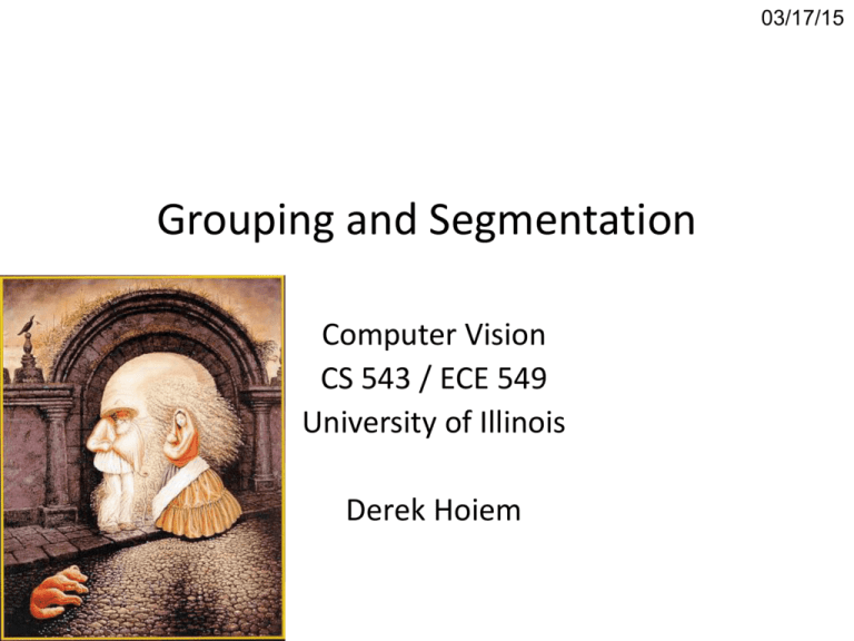
03/17/15
Grouping and Segmentation
Computer Vision
CS 543 / ECE 549
University of Illinois
Derek Hoiem
Today’s class
• Segmentation and grouping
– Gestalt cues
– By clustering (mean-shift)
– By boundaries (watershed)
• Superpixels and multiple segmentations
Gestalt psychology or gestaltism
German: Gestalt - "form" or "whole”
Berlin School, early 20th century
Kurt Koffka, Max Wertheimer, and Wolfgang Köhler
View of brain:
• whole is more than the sum of its parts
• holistic
• parallel
• analog
• self-organizing tendencies
Slide from S. Saverese
Gestaltism
The Muller-Lyer illusion
We perceive the interpretation, not the
senses
Principles of perceptual organization
From Steve Lehar: The Constructive Aspect of Visual Perception
Principles of perceptual organization
Gestaltists do not believe in coincidence
Emergence
Grouping by invisible completion
From Steve Lehar: The Constructive Aspect of Visual Perception
Grouping involves global interpretation
From Steve Lehar: The Constructive Aspect of Visual Perception
Grouping involves global interpretation
From Steve Lehar: The Constructive Aspect of Visual Perception
Gestalt cues
• Good intuition and basic principles for
grouping
• Basis for many ideas in segmentation and
occlusion reasoning
• Some (e.g., symmetry) are difficult to
implement in practice
Image segmentation
Goal: Group pixels into meaningful or
perceptually similar regions
Segmentation for efficiency: “superpixels”
[Felzenszwalb and Huttenlocher 2004]
[Hoiem et al. 2005, Mori 2005]
[Shi and Malik 2001]
Segmentation for feature support
50x50 Patch
50x50 Patch
Segmentation for object proposals
“Selective Search” [Sande, Uijlings et al. ICCV 2011, IJCV 2013]
[Endres Hoiem ECCV 2010, IJCV 2014]
• Object proposals
• Superpixels, proposals, multiple
segmentations
Segmentation as a result
Rother et al. 2004
Major processes for segmentation
• Bottom-up: group tokens with similar features
• Top-down: group tokens that likely belong to
the same object
[Levin and Weiss 2006]
Segmentation using clustering
• Kmeans
• Mean-shift
Feature Space
Source: K. Grauman
K-means clustering using intensity alone and color alone
Image
Clusters on intensity
Clusters on color
K-Means pros and cons
• Pros
– Simple and fast
– Easy to implement
• Cons
– Need to choose K
– Sensitive to outliers
• Usage
– Rarely used for pixel
segmentation
Mean shift segmentation
D. Comaniciu and P. Meer, Mean Shift: A Robust Approach toward Feature Space Analysis, PAMI 2002.
• Versatile technique for clustering-based
segmentation
Mean shift algorithm
• Try to find modes of this non-parametric
density
Kernel density estimation
Kernel
Estimated
density
Data (1-D)
Kernel density estimation
Kernel density estimation function
Gaussian kernel
Mean shift
Region of
interest
Center of
mass
Mean Shift
vector
Slide by Y. Ukrainitz & B. Sarel
Mean shift
Region of
interest
Center of
mass
Mean Shift
vector
Slide by Y. Ukrainitz & B. Sarel
Mean shift
Region of
interest
Center of
mass
Mean Shift
vector
Slide by Y. Ukrainitz & B. Sarel
Mean shift
Region of
interest
Center of
mass
Mean Shift
vector
Slide by Y. Ukrainitz & B. Sarel
Mean shift
Region of
interest
Center of
mass
Mean Shift
vector
Slide by Y. Ukrainitz & B. Sarel
Mean shift
Region of
interest
Center of
mass
Mean Shift
vector
Slide by Y. Ukrainitz & B. Sarel
Mean shift
Region of
interest
Center of
mass
Slide by Y. Ukrainitz & B. Sarel
Computing the Mean Shift
Simple Mean Shift procedure:
• Compute mean shift vector
•Translate the Kernel window by m(x)
 n

 x - xi 2 
  xi g 


 h 
 i 1



m ( x)  
 x
2
 n  x - xi 

  g  h 

i 1




Slide by Y. Ukrainitz & B. Sarel
Real Modality Analysis
Attraction basin
• Attraction basin: the region for which all
trajectories lead to the same mode
• Cluster: all data points in the attraction
basin of a mode
Slide by Y. Ukrainitz & B. Sarel
Attraction basin
Mean shift clustering
• The mean shift algorithm seeks modes of the
given set of points
1. Choose kernel and bandwidth
2. For each point:
a)
b)
c)
d)
Center a window on that point
Compute the mean of the data in the search window
Center the search window at the new mean location
Repeat (b,c) until convergence
3. Assign points that lead to nearby modes to the
same cluster
Segmentation by Mean Shift
•
•
•
•
•
Compute features for each pixel (color, gradients, texture, etc); also store
each pixel’s position
Set kernel size for features Kf and position Ks
Initialize windows at individual pixel locations
Perform mean shift for each window until convergence
Merge modes that are within width of Kf and Ks
Mean shift segmentation results
http://www.caip.rutgers.edu/~comanici/MSPAMI/msPamiResults.html
http://www.caip.rutgers.edu/~comanici/MSPAMI/msPamiResults.html
Mean-shift: other issues
• Speedups
– Binned estimation – replace points within some “bin” by
point at center with mass
– Fast search of neighbors – e.g., k-d tree or approximate NN
– Update all windows in each iteration (faster convergence)
• Other tricks
– Use kNN to determine window sizes adaptively
• Lots of theoretical support
D. Comaniciu and P. Meer, Mean Shift: A Robust Approach toward
Feature Space Analysis, PAMI 2002.
Mean shift pros and cons
• Pros
–
–
–
–
Good general-purpose segmentation
Flexible in number and shape of regions
Robust to outliers
General mode-finding algorithm (useful for other problems such
as finding most common surface normals)
• Cons
– Have to choose kernel size in advance
– Not suitable for high-dimensional features
• When to use it
– Oversegmentation
– Multiple segmentations
– Tracking, clustering, filtering applications
• D. Comaniciu, V. Ramesh, P. Meer: Real-Time Tracking of Non-Rigid
Objects using Mean Shift, Best Paper Award, IEEE Conf. Computer Vision
and Pattern Recognition (CVPR'00), Hilton Head Island, South Carolina,
Vol. 2, 142-149, 2000
Mean-shift reading
• Nicely written mean-shift explanation (with
math)
http://saravananthirumuruganathan.wordpress.com/2010/04/01/introduction-to-mean-shiftalgorithm/
• Includes .m code for mean-shift clustering
• Mean-shift paper by Comaniciu and Meer
http://www.caip.rutgers.edu/~comanici/Papers/MsRobustApproach.pdf
• Adaptive mean shift in higher dimensions
http://mis.hevra.haifa.ac.il/~ishimshoni/papers/chap9.pdf
Superpixel algorithms
• Goal is to divide the image into a large
number of regions, such that each regions lie
within object boundaries
• Examples
– Watershed
– Felzenszwalb and Huttenlocher graph-based
– Turbopixels
– SLIC
Watershed algorithm
Watershed segmentation
Image
Gradient
Watershed boundaries
Meyer’s watershed segmentation
1. Choose local minima as region seeds
2. Add neighbors to priority queue, sorted by
value
3. Take top priority pixel from queue
1. If all labeled neighbors have same label, assign
that label to pixel
2. Add all non-marked neighbors to queue
4. Repeat step 3 until finished (all remaining
pixels in queue are on the boundary)
Matlab: seg = watershed(bnd_im)
Meyer 1991
Simple trick
• Use Gaussian or median filter to reduce number of
regions
Watershed usage
• Use as a starting point for hierarchical
segmentation
– Ultrametric contour map (Arbelaez 2006)
• Works with any soft boundaries
– Pb (w/o non-max suppression)
– Canny (w/o non-max suppression)
– Etc.
Watershed pros and cons
• Pros
– Fast (< 1 sec for 512x512 image)
– Preserves boundaries
• Cons
– Only as good as the soft boundaries (which may be slow to
compute)
– Not easy to get variety of regions for multiple segmentations
• Usage
– Good algorithm for superpixels, hierarchical segmentation
Felzenszwalb and Huttenlocher: GraphBased Segmentation
http://www.cs.brown.edu/~pff/segment/
+ Good for thin regions
+ Fast
+ Easy to control coarseness of segmentations
+ Can include both large and small regions
- Often creates regions with strange shapes
- Sometimes makes very large errors
Turbo Pixels: Levinstein et al. 2009
http://www.cs.toronto.edu/~kyros/pubs/09.pami.turbopixels.pdf
Tries to preserve boundaries like watershed but to produce more regular regions
SLIC
(Achanta et al. PAMI 2012)
http://infoscience.epfl.ch/record/177415/files/Superpixel_PAMI2011-2.pdf
1. Initialize cluster centers on
pixel grid in steps S
- Features: Lab color, x-y position
2. Move centers to position in
3x3 window with smallest
gradient
3. Compare each pixel to cluster
center within 2S pixel distance
and assign to nearest
4. Recompute cluster centers as
mean color/position of pixels
belonging to each cluster
5. Stop when residual error is
small
+ Fast 0.36s for 320x240
+ Regular superpixels
+ Superpixels fit boundaries
- May miss thin objects
- Large number of superpixels
Choices in segmentation algorithms
• Oversegmentation
– Watershed + Pb  my favorite
– Felzenszwalb and Huttenlocher 2004  my favorite
http://www.cs.brown.edu/~pff/segment/
– SLIC  good recent option
– Turbopixels
– Mean-shift
• Larger regions
–
–
–
–
Hierarchical segmentation (e.g., from Pb)  my favorite
Normalized cuts
Mean-shift
Seed + graph cuts (discussed later)
Multiple segmentations
• When creating regions for pixel classification
or object detection, don’t commit to one
partitioning
• Strategies:
– Hierarchical segmentation
• Occlusion boundaries hierarchy: Hoiem et al. IJCV
2011 (uses trained classifier to merge)
• Pb+watershed hierarchy: Arbeleaz et al. CVPR
2009
• Selective search: FH + agglomerative clustering
– Vary segmentation parameters
• E.g., multiple graph-based segmentations or
mean-shift segmentations
– Region proposals
• Propose seed superpixel, try to segment out
object that contains it (Endres Hoiem ECCV 2010,
Carreira Sminchisescu CVPR 2010)
Things to remember
• Gestalt cues and principles of organization
• Uses of segmentation
–
–
–
–
Efficiency
Better features
Propose object regions
Want the segmented object
• Mean-shift segmentation
– Good general-purpose segmentation method
– Generally useful clustering, tracking technique
• Watershed segmentation
– Good for hierarchical segmentation
– Use in combination with boundary prediction
Next class: EM algorithm
• Make sure to bring something to take notes
(will include a long derivation)