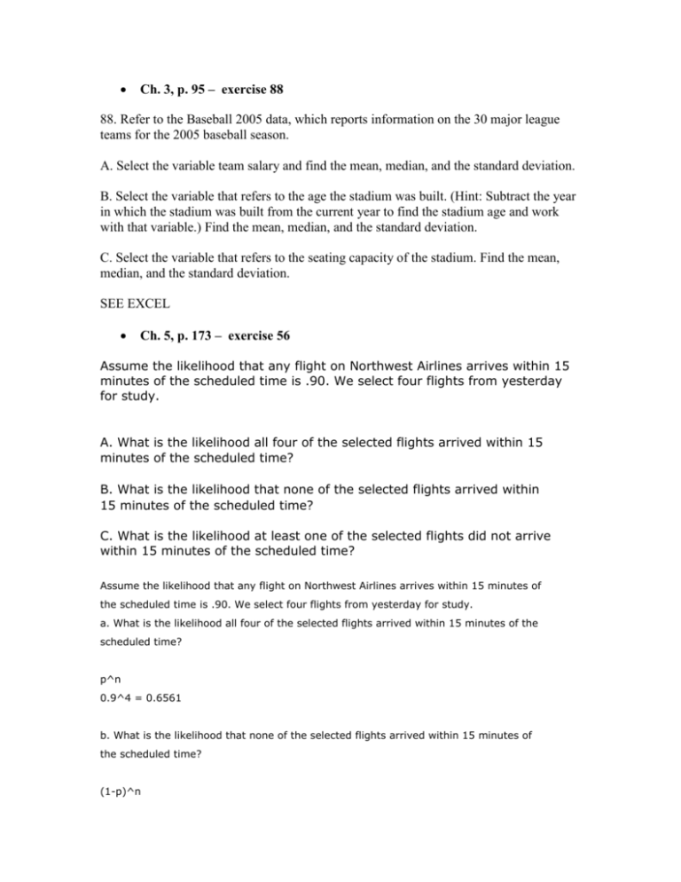

Ch. 3, p. 95 – exercise 88
88. Refer to the Baseball 2005 data, which reports information on the 30 major league
teams for the 2005 baseball season.
A. Select the variable team salary and find the mean, median, and the standard deviation.
B. Select the variable that refers to the age the stadium was built. (Hint: Subtract the year
in which the stadium was built from the current year to find the stadium age and work
with that variable.) Find the mean, median, and the standard deviation.
C. Select the variable that refers to the seating capacity of the stadium. Find the mean,
median, and the standard deviation.
SEE EXCEL

Ch. 5, p. 173 – exercise 56
Assume the likelihood that any flight on Northwest Airlines arrives within 15
minutes of the scheduled time is .90. We select four flights from yesterday
for study.
A. What is the likelihood all four of the selected flights arrived within 15
minutes of the scheduled time?
B. What is the likelihood that none of the selected flights arrived within
15 minutes of the scheduled time?
C. What is the likelihood at least one of the selected flights did not arrive
within 15 minutes of the scheduled time?
Assume the likelihood that any flight on Northwest Airlines arrives within 15 minutes of
the scheduled time is .90. We select four flights from yesterday for study.
a. What is the likelihood all four of the selected flights arrived within 15 minutes of the
scheduled time?
p^n
0.9^4 = 0.6561
b. What is the likelihood that none of the selected flights arrived within 15 minutes of
the scheduled time?
(1-p)^n
(1-0.9)^4
0.1^4
= 0.0001
c. What is the likelihood at least one of the selected flights did not arrive within 15 minutes
of the scheduled time?
at least one = 1 - prob(all arrived)
= 1 - 0.6561
= 0.3439

Ch. 6, p. 217 – exercise 64
An internal study by the Technology Services department at Lahey Electronics revealed
company employees receive an average of two emails per hour. Assume the arrival of
these emails is approximated by the Poisson distribution.
A. What is the probability Linda Lahey, company president, received exactly 1 email
between 4 P.M. and 5 P.M. yesterday?
B. What is the probability she received 5 or more email during the same period?
C. What is the probability she did not receive any email during the period?
The average is 2 per hour.
I'll use the Poisson calculator here: http://stattrek.com/Tables/poisson.aspx
a. What is the probability Linda Lahey, company president, received exactly 1 email between 4
P.M. and 5 P.M. yesterday?
0.270670566473225
Using the formula:
f(x) = e-λλx / x!
= e^(-2)*(2)^1 / 1
same result as the above with a calculator
b. What is the probability she received 5 or more email during the same period?
= 1 - 4 or less
= 1 - 0.947346982656289
= 0.052653017343711
Or with the formula:
1 - e^(-2)*(2)^0 / 1 - e^(-2)*(2)^1 / 1 - e^(-2)*(2)^2 / 2 - e^(-2)*(2)^3 / 6 - e^(2)*(2)^4 / 24
which evaluates to the above
c. What is the probability she did not receive any email during the period?
0.135335283236613
Using the formula:
f(x) = e-λλx / x!
= e^(-2)*(2)^0 / 1
Again, the same result as the above...

Ch. 7, p. 249 – exercise 50
Fast Service Truck Lines uses the Ford Super Duty F-750 exclusively.
Management made a study of the maintenance costs and determined the
number of miles traveled during the year followed the normal distribution.
The mean of the distribution was 60,000 miles and the standard deviation
2,000 miles.
A. What percent of the Ford Super Duty F-750s logged 65,200 miles
or more?
B. What percent of the trucks logged more than 57,060 but less
than 58,280 miles?
C. What percent of the Fords traveled 62,000 miles or less during
the year?
D. Is it reasonable to conclude that any of the trucks were driven
more than 70,000 miles? Explain.
I'll be using this z table: http://davidmlane.com/hyperstat/z_table.html
a. What percent of the Ford Super Duty F-750s logged 65,200 miles or more?
z(65200) = (65200-60000)/2000 = 2.6
prob(z > 2.6)
= 0.466%
b. What percent of the trucks logged more than 57,060 but less than 58,280 miles?
z(57060) = (57060-60000)/2000 = -1.47
z(58280) = (58280-60000)/2000 = -0.86
prob(-1.47 < z < -0.86)
= 12.41%
c. What percent of the Fords traveled 62,000 miles or less during the year?
z(62000) = (62000-60000)/2000 = 1
prob(z < 1)
= 84.13%
d. Is it reasonable to conclude that any of the trucks were driven more than 70,000 miles?
Explain.
z(70000) = (70000-60000)/2000 = 5
prob(z > 5)
= about 0% (it's greater than 0, but the z table shows it as 0)
It is not reasonable, since the proportion of a population that's more than 5 standard
deviations above the mean is basically 0.

Ch. 8, p. 288 – exercise 38
The mean amount purchased by a typical customer at Churchill's
Grocery Store is $23.50 with a standard deviation of $5.00. Assume
the distribution of amounts purchased follows the normal distribution.
For a sample of 50 customers, answer the following questions.
A. What is the likelihood the sample mean is at least
$25.00?
B. What is the likelihood the sample mean is greater
than $22.50 but less than $25.00?
C. Within what limits will 90 percent of the sample
means occur?
a. What is the likelihood the sample mean is at least $25.00?
z = (25-23.5)/(5/sqrt(50))
z = 2.12132
prob(z > 2.12132)
= 0.0169
b. What is the likelihood the sample mean is greater than $22.50 but less than $25.00?
z(22.5) = (22.5-23.5)/(5/sqrt(50)) = -1.4142
prob(-1.4142 < z < 2.12132)
= 0.9044
c. Within what limits will 90 percent of the sample means occur?
z = +/-1.6449
The interval goes from:
mean - z*sd/sqrt(N) to mean + z*sd/sqrt(N)
23.5 - 1.6449*5/sqrt(50) to 23.5 + 1.6449*5/sqrt(50)
22.3369 to 24.6631

Ch. 9, p. 321 – exercise 54
Families USA, a monthly magazine that discusses issues related to health and health
costs, surveyed 20 of its subscribers. It found that the annual health insurance premiums
for a family with coverage through an employer averaged $10,979. The standard
deviation of the sample was $1,000.
A. Based on this sample information, develop a 90 percent confidence interval for
the population mean yearly premium.
B. How large a sample is needed to find the population mean within $250 at 99
percent confidence?
a. Based on this sample information, develop a 90 percent confidence interval for the
population mean yearly premium.
The t value for df = n-1 = 19, with 90% confidence is:
1.7291
The interval goes from:
mean - t*sd/sqrt(N) to mean + t*sd/sqrt(N)
10979 - 1.7291*1000/sqrt(20) to 10979 - 1.7291*1000/sqrt(20)
With a calculator:
10592.36 to 11365.64
b. How large a sample is needed to find the population mean within $250 at 99 percent
confidence?
The z value for 99% confidence is 2.5758
The formula for sample size is:
N = (z*sd/E)^2
N = (2.5758*1000/250)^2
N = 106.16
Round up to:
N = 107

Ch. 10, p. 362 – exercise 42
During recent seasons, Major League Baseball has been criticized for the
length of the games. A report indicated that the average game lasts 3 hours
and 30 minutes. A sample of 17 games revealed the following times to
completion. (Note that the minutes have been changed to fractions of hours,
so that a game that lasted 2 hours and 24 minutes is reported at 2.40
hours.)
2.98
2.40
2.70
2.25
3.23
3.17
2.93
3.18
2.38
3.75
3.20
3.27
2.52
2.58
4.45
2.45
2.80
Can we conclude that the mean time for a game is less than 3.50 hours?
Use the .05 significance level.
H0: game length is >= 3.5 hours
Ha: game length is < 3.5 hours
mean = 2.9553
stdev = 0.5596
Get the t test statistic:
t = (x-mu)/(stdev/sqrt(N))
t = (2.9553-3.5)/(0.5596/sqrt(17))
t = -4.0133
Get the critical value for df = N-1 = 16, one tail, alpha is 0.05:
-1.7459
Since our test statistic is much lower than the critical value, we reject the null hypothesis.
There is enough evidence to conclude that games are shorter than 3.50 hours.

Ch. 11, p. 402 – exercise 58
The amount of income spent on housing is an important component of the
cost of living. The total costs of housing for homeowners might include
mortgage payments, property taxes, and utility costs (water, heat,
electricity). An economist selected a sample of 20 homeowners in New
England and then calculated these total housing costs as a percent of
monthly income, five years ago and now. The information is reported below.
Is it reasonable to conclude the percent is less now than five years ago?
Home Owner
1
2
3
4
5
6
7
8
9
10
11
12
13
14
15
16
17
18
19
20
Five years ago
17%
20
29
43
36
43
45
19
49
49
35%
16
23
33
44
44
28
29
39
22
Now
10%
39
37
27
12
41
24
26
28
26
32%
32
21
12
40
42
22
19
35
12
SEE EXCEL

Ch. 12, p. 445 – exercise 42
Martin Motors has in stock three cars of the same make and model. The
president would like to compare the gas consumption of the three cars
(labeled car A, car B, and car C) using four different types of gasoline.
For each trial, a gallon of gasoline was added to an empty tank, and the car
was driven until it ran out of gas. The following table shows the number of
miles driven in each trial.
Distance (miles)
of Gasoline
Car A
Car B
Car C
Regular
22.4
20.8
21.5
Super regular
17.0
19.4
20.7
Unleaded
19.2
20.2
21.2
Premium unleaded
20.3
18.6
20.4
Using the .05 level of significance:
A. Is there a difference among types of gasoline?
B. Is there a difference in the cars?
SEE EXCEL

Ch. 13, pp. 499 – exercise 37
A regional commuter airline selected a random sample of 25 flights and
found that the correlation between the number of passengers and the total
weight, in pounds, of luggage stored in the luggage compartment is 0.94.
Using the .05 significance level, can we conclude that there is a positive
association between the two variables?
SEE EXCEL

Ch. 14, pp. 548-49 – exercise 17
The district manager of Jasons, a large discount electronics chain, is
investigating why certain stores in her region are performing better than
others. She believes that three factors are related to total sales: the number
of competitors in the region, the population in the surrounding area, and the
amount spent on advertising. From her district, consisting of several hundred
stores, she selects a random sample of 30 stores. For each store she
gathered the following information.
Y=
total sales last year (in $ thousands).
X1 =
number of competitors in the region.
X2 =
population of the region (in millions).
X3 =
advertising expense (in $ thousands).
The sample data were run on MINITAB, with the following results.
Analysis of
Variance
Source
Regression
Error
DF
3
26
Total
Predictor
Constant
X1
X2
X3
29
Coef
14.00
-1.00
30.00
0.20
SS
MS
3050.00 1016.67
2200.000 84.62
Â
5250.000
StDev
t-ratio
7.00
2.00
0.70
2.00
5.20
5.77
0.08
2.50
A. What are the estimated sales for the Bryne store,
which has four competitors, a regional population of
0.4 (400,000), and advertising expense of 30
($30,000)?
B. Compute the R2 value.
C. Compute the multiple standard error of estimate.
D. Conduct a global test of hypothesis to determine
whether any of the regression coefficients are not
equal to zero. Use the .05 level of significance.
E. Conduct tests of hypotheses to determine which of
the independent variables have significant
regression coefficients. Which variables would you
consider eliminating? Use the .05 significance level.
a. What are the estimated sales for the Bryne store, which has four competitors, a
regional population of 0.4 (400,000), and advertising expense of 30 ($30,000)?
Use the regression:
14 - 1*4 + 30*0.4 + 0.2*30
= 28
So the sales would be $28000, since the regression gives the value in thousands
b. Compute the value of r^2.
ssr/sst
= 3050/5250
= 0.58095
c. Compute the multiple standard error of estimate.
sqrt(mse)
= sqrt(84.62)
= 9.1989
d. Conduct a global test of hypothesis to determine whether any of the regression coefficients
are not equal to zero. Use the .05 level of significance.
H0: coeffs are zero
Ha: coeffs are not zero
F = 1016.67/84.62
= 12.01454
The critical value, from an F table, with df = 3, 26 is: 2.975
The test statistic is much higher, so we reject the null.
At least one coefficient is non zero.
e. Conduct tests of hypotheses to determine which of the independent variables have
significant regression coefficien
Each hypothesis looks like this:
H0: coefficient for Xn is 0
Ha: coefficient for Xn is non zero
The critical T value, from a table, is 2.056
The t value for X1 is not outside that range, so we don't reject.
The t value for X2 and X3 are outside, so we reject.
X2 and X3 are significant.

Ch. 17, p. 664-65 – exercise 22
Banner Mattress and Furniture Company wishes to study the number of
credit applications received per day for the last 300 days. The information is
reported on the next page.
Number of Credit Applications
Frequency (Number of Days)
0
50
1
77
2
81
3
48
4
31
5 or more
13
To interpret, there were 50 days on which no credit applications were
received, 77 days on which only one application was received, and so on.
Would it be reasonable to conclude that the population distribution is Poisson
with a mean of 2.0? Use the .05 significance level. Hint: To find the expected
frequencies use the Poisson distribution with a mean of 2.0. Find the
probability of exactly one success given a Poisson distribution with a mean of
2.0. Multiply this probability by 300 to find the expected frequency for the
number of days in which there was exactly one application. Determine the
expected frequency for the other days in a similar manner.
SEE EXCEL