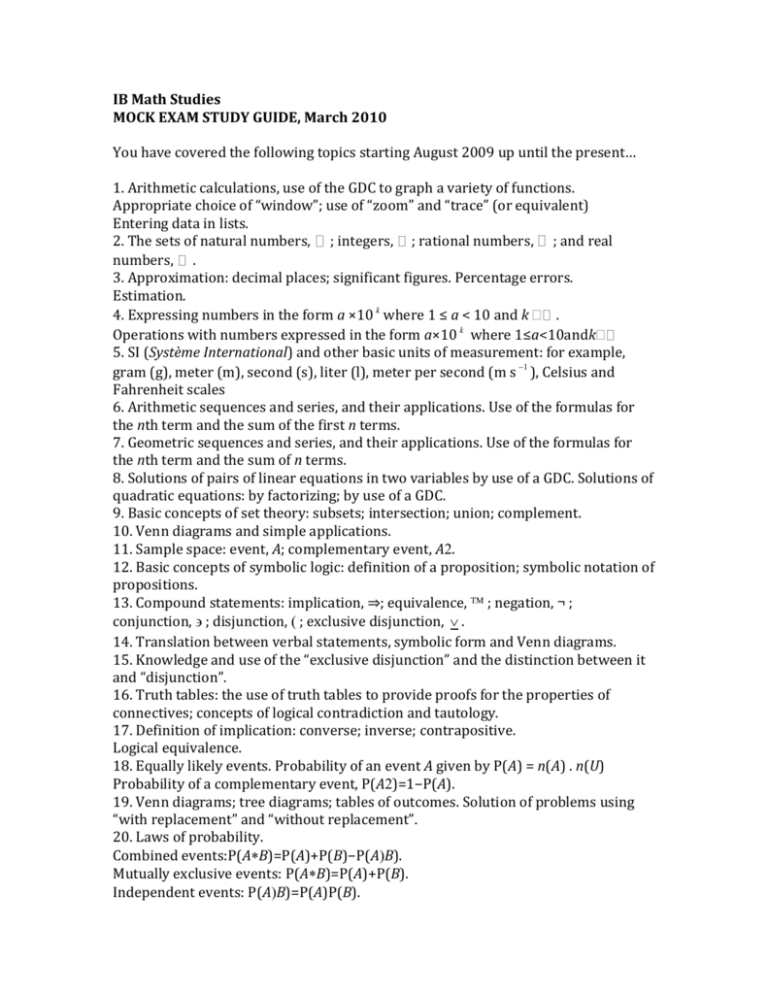
IB Math Studies
MOCK EXAM STUDY GUIDE, March 2010
You have covered the following topics starting August 2009 up until the present…
1. Arithmetic calculations, use of the GDC to graph a variety of functions.
Appropriate choice of “window”; use of “zoom” and “trace” (or equivalent)
Entering data in lists.
2. The sets of natural numbers, ; integers, ; rational numbers, ; and real
numbers, .
3. Approximation: decimal places; significant figures. Percentage errors.
Estimation.
4. Expressing numbers in the form a ×10 k where 1 ≤ a < 10 and k  .
Operations with numbers expressed in the form a×10 k where 1≤a<10andk
5. SI (Système International) and other basic units of measurement: for example,
gram (g), meter (m), second (s), liter (l), meter per second (m s 1 ), Celsius and
Fahrenheit scales
6. Arithmetic sequences and series, and their applications. Use of the formulas for
the nth term and the sum of the first n terms.
7. Geometric sequences and series, and their applications. Use of the formulas for
the nth term and the sum of n terms.
8. Solutions of pairs of linear equations in two variables by use of a GDC. Solutions of
quadratic equations: by factorizing; by use of a GDC.
9. Basic concepts of set theory: subsets; intersection; union; complement.
10. Venn diagrams and simple applications.
11. Sample space: event, A; complementary event, A.
12. Basic concepts of symbolic logic: definition of a proposition; symbolic notation of
propositions.
13. Compound statements: implication, ⇒; equivalence,  ; negation, ¬ ;
conjunction,  ; disjunction,  ; exclusive disjunction,  .
14. Translation between verbal statements, symbolic form and Venn diagrams.
15. Knowledge and use of the “exclusive disjunction” and the distinction between it
and “disjunction”.
16. Truth tables: the use of truth tables to provide proofs for the properties of
connectives; concepts of logical contradiction and tautology.
17. Definition of implication: converse; inverse; contrapositive.
Logical equivalence.
18. Equally likely events. Probability of an event A given by P(A) = n(A) . n(U)
Probability of a complementary event, P(A)=1−P(A).
19. Venn diagrams; tree diagrams; tables of outcomes. Solution of problems using
“with replacement” and “without replacement”.
20. Laws of probability.
Combined events:P(AB)=P(A)+P(B)−P(AB).
Mutually exclusive events: P(AB)=P(A)+P(B).
Independent events: P(AB)=P(A)P(B).
P A  B 
P B 
21. Concept of a function as a mapping. Domain and range. Mapping diagrams.
22. Linear functions and their graphs, for example, f : x
mx + c .
2
23. The graph of the quadratic function: f(x)=ax +bx+c; Properties of symmetry;
vertex; intercepts.
24. The exponential expression: a b ; b 
Graphs and properties of exponential
x
x
x
functions. f (x) = a ; f (x) = a ; f(x)=ka +c; k,a,c,λ 
Growth and decay; basic concepts of asymptotic behavior.
25. Graphs and properties of the sine and cosine functions:
f (x) = asinbx + c ; f(x)=acosbx+c; a,b,c, . Amplitude and period.
26. Accurate graph drawing.
27. Use of a GDC to sketch and analyze some simple, unfamiliar functions.
28. Use of a GDC to solve equations involving simple combinations of some simple,
unfamiliar functions.
29. Coordinates in two dimensions: points; lines; midpoints. Distances between
points.
30. Equation of a line in two dimensions: the forms y=mx+c and ax+by+d =0.
Gradient; intercepts; Points of intersection of lines; parallel lines; perpendicular
lines.
31. Right-angled trigonometry. Use of the ratios of sine, cosine and tangent.
a
b
c
32. The sine rule:
=
=
; The cosine rule a 2 =b 2 +c 2 −2bccosA;
sin A sin B sin C
2
2
2
1
b c a
cos A 
; Area of a triangle: ab sin C
2
2bc
33. Geometry of three-dimensional shapes: cuboid; prism; pyramid; cylinder;
sphere; hemisphere; cone. Lengths of lines joining vertices with vertices, vertices
with midpoints and midpoints with midpoints; sizes of angles between two lines
and between lines and planes.
34. Classification of data as discrete or continuous.
35. Simple discrete data: frequency tables; frequency polygons.
36. Grouped discrete or continuous data: frequency tables; mid-interval values;
upper and lower boundaries. Frequency histograms. Stem-and-leaf diagrams.
37. Cumulative frequency tables for grouped discrete data and for grouped
continuous data; cumulative frequency curves. Box and whisker plots (box plots).
Percentiles; quartiles.
38. Measures of central tendency. For simple discrete data: mean; median; mode.
For grouped discrete and continuous data: approximate mean; modal group; 50th
percentile.
39. Measures of dispersion: range; interquartile range; standard deviation.
40. Scatter diagrams; line of best fit, by eye, passing through the mean point.
Bivariate data: the concept of correlation. Pearson’s product–moment correlation
Conditional probability: P( A | B) =
coefficient: Use of the formula r =
s xy
sx sy
; Interpretation of positive, zero and negative
correlations.
41. The regression line for y on x: use of the formula y  y 
sxy
sx2
x  x 
Use of the regression line for prediction purposes.
42. The  2 test for independence: formulation of null and alternative hypotheses;
significance levels; contingency tables; expected frequencies; use of the formula
2
f o  fe 

2
; degrees of freedom; use of tables for critical values; p-values.
 calc
fe