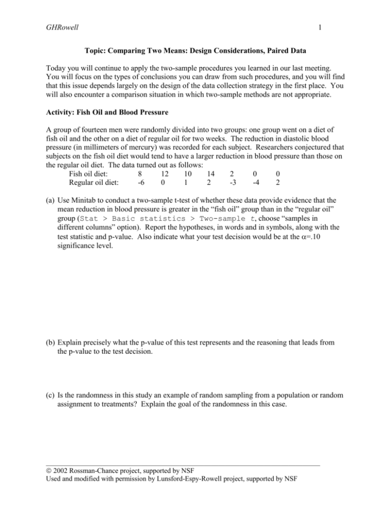
GHRowell
1
Topic: Comparing Two Means: Design Considerations, Paired Data
Today you will continue to apply the two-sample procedures you learned in our last meeting.
You will focus on the types of conclusions you can draw from such procedures, and you will find
that this issue depends largely on the design of the data collection strategy in the first place. You
will also encounter a comparison situation in which two-sample methods are not appropriate.
Activity: Fish Oil and Blood Pressure
A group of fourteen men were randomly divided into two groups: one group went on a diet of
fish oil and the other on a diet of regular oil for two weeks. The reduction in diastolic blood
pressure (in millimeters of mercury) was recorded for each subject. Researchers conjectured that
subjects on the fish oil diet would tend to have a larger reduction in blood pressure than those on
the regular oil diet. The data turned out as follows:
Fish oil diet:
8
12
10
14
2
0
0
Regular oil diet:
-6
0
1
2
-3
-4
2
(a) Use Minitab to conduct a two-sample t-test of whether these data provide evidence that the
mean reduction in blood pressure is greater in the “fish oil” group than in the “regular oil”
group (Stat > Basic statistics > Two-sample t, choose “samples in
different columns” option). Report the hypotheses, in words and in symbols, along with the
test statistic and p-value. Also indicate what your test decision would be at the =.10
significance level.
(b) Explain precisely what the p-value of this test represents and the reasoning that leads from
the p-value to the test decision.
(c) Is the randomness in this study an example of random sampling from a population or random
assignment to treatments? Explain the goal of the randomness in this case.
______________________________________________________________________________
 2002 Rossman-Chance project, supported by NSF
Used and modified with permission by Lunsford-Espy-Rowell project, supported by NSF
GHRowell
2
Activity: Bumpus Data on Natural Selection
A scientist named Bumpus conducted an investigation of natural selection by comparing
measurements on two groups of sparrows: one group that had survived an unusually harsh winter
storm and another group that perished in the storm. One of the variables measured was the
length of the humerus (arm bone, measured in inches); the data appear in bumpus.mtw.
(a) Examine visual displays (Graph > Dotplot, Graph > Boxplot) and calculate
descriptive statistics (Stat > Basic statistics > Display descriptive
statistics) for comparing the humerus lengths between the two groups. Comment on
the similarities and differences between the two distributions (shape, center, spread).
(b) State the appropriate hypotheses, in symbols and in words, for testing the scientist’s
conjecture that humerus lengths would tend to be longer in sparrows that survived the storm.
(c) Use Minitab to conduct this test. Report the test statistic and p-value.
(d) Do the sample means of these two groups differ significantly at the =.05 level? Summarize
your conclusion, and explain how it follows from the test.
(e) Even if the p-value were tiny and so the difference were extremely significant, would you be
able to legitimately conclude that the physical advantage caused those sparrows to survive
the storm? Explain.
______________________________________________________________________________
 2002 Rossman-Chance project, supported by NSF
Used and modified with permission by Lunsford-Espy-Rowell project, supported by NSF
GHRowell
3
Conclusions about cause-and-effect can not be drawn from observational studies, in which
researchers passively record information without actively assigning treatments to subjects. With
such studies one can never be sure that a confounding variable, not the specific variable being
studied, might be responsible for any differences in the response variable. To balance out the
effects of potentially confounding variables, one can randomly assign subjects to treatment
groups. With a randomized controlled experiment, one can legitimately make inferences about
cause-and-effect conclusions.
Activity: Foreign Language and SAT Scores
Students who study a foreign language in high school typically perform better on the Verbal
portion of the SAT than students who do not study a foreign language.
(a) According to this statement, if the Verbal SAT scores of a large random sample of students
studying a foreign language were compared to those of a large random sample of students not
studying a foreign language, would you expect the p-value to be large or small? Explain.
(b) Suggest a confounding variable that could affect both interest in studying a foreign language
and Verbal SAT score.
(c) Is this situation an observational study or a controlled experiment? Explain.
(d) How would you go about conducting a randomized controlled experiment to address the
question of whether foreign language study tends to improve students’ Verbal SAT scores?
What are the practical or ethical impediments to conducting such an experiment? Explain.
______________________________________________________________________________
 2002 Rossman-Chance project, supported by NSF
Used and modified with permission by Lunsford-Espy-Rowell project, supported by NSF
GHRowell
4
Activity: Marriage Ages
Suppose that you want to investigate whether husbands tend to be older than wives on the
average. A student went to the county courthouse and recorded the ages appearing on marriage
licenses for a sample of 24 couples; the data can be found in marriage.mtw (c2 and c3).
(a) Use Minitab to test whether these sample data provide evidence that the mean age of a male
applicant for a marriage license is higher than that of a female applicant. Report the
hypotheses (in symbols and in words), the test statistic, and p-value. Also state and explain
your conclusion.
The two-sample t-test is completely inappropriate in this situation, because these samples of
marriage ages are not independent. These data pertain to couples, and it seems reasonable to
believe that the age of one partner is related to the age of the other.
(b) Use Minitab to examine a scatterplot of husband’s age vs. wife’s age (Graph > Plot,
with husband on y axis and wife on x axis, or MTB> plot c2 c3). Does there appear to
be an association between husband’s age and wife’s age, or do they seem to be independent
after all? Explain.
With paired data it makes sense to analyze the differences between the two groups within each
pair and then proceed with a one-sample t-test.
(c) Use Minitab to calculate the differences (MTB> let c4=c2-c3) and then to examine
visual displays of this distribution of age differences. Comment on that distribution (shape,
center, spread).
(d) Use Minitab to apply a one-sample t-test on the resulting data (Stat > Basic
statistics > One-sample t). Report the hypotheses, in words and in symbols, as
well as the test statistic, p-value, and your conclusion.
This procedure is called a paired t-test.
______________________________________________________________________________
 2002 Rossman-Chance project, supported by NSF
Used and modified with permission by Lunsford-Espy-Rowell project, supported by NSF
GHRowell
5
(e) Have the test statistic and p-value changed much from the two-sample test?
(f) To see why the test statistic has changed so much, calculate the means and standard
deviations of these three variables (MTB> describe c2 c3 c4) and record them in the
table below. Use these statistics to suggest why the test statistic based on the sample of
differences is so much larger than that based on independent samples. [Hint: Think about
whether the numerator or denominator in the test statistic calculation has changed.]
husband’s age
wife’s age
difference in ages
mean
Standard deviation
The key advantage of pairing, also known as blocking, is that it reduces variability. The
difference in means of 1.875 years does not look very significant compared to standard
deviations of the marriages ages (14.56 and 13.56), but it is much more significant when
compared to the standard deviation of the differences (4.812).
(g) Use Minitab to produce a 90% confidence interval for the mean difference in ages among all
married couples. Comment on the importance of whether this interval includes the value
zero.
______________________________________________________________________________
 2002 Rossman-Chance project, supported by NSF
Used and modified with permission by Lunsford-Espy-Rowell project, supported by NSF