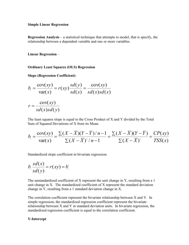
Simple Linear Regression
Regression Analysis – a statistical technique that attempts to model, that is specify, the
relationship between a dependent variable and one or more variables.
Linear Regression –
Ordinary Least Squares (OLS) Regression
Slope (Regression Coefficient):
b 
cov( xy)
sd ( y )
cov( xy)
 r ( xy)

var( x)
sd ( x) sd ( x) sd ( x)
r
cov( xy )
sd ( x) sd ( y )
1
The least squares slope is equal to the Cross Product of X and Y divided by the Total
Sum of Squared Deviations of X from its Mean.
b
1
cov( xy)  ( X  X )(Y  Y ) / n  1  ( X  X )(Y  Y ) CP( xy)



var( x)
(
X

X
)
/
n

1
(
X

X
)
TSS ( x)


2
2
Standardized slope coefficient in bivariate regression.
b
1
sd ( x)
 r ( xy)  b
sd ( y )
*
1
The unstandardized coefficient of X represent the unit change in Y, resulting from a 1
unit change in X. The standardized coefficient of X represent the standard deviation
change in Y, resulting from a 1 standard deviation change in X.
The correlation coefficient represent the bivariate relationship between X and Y. In
simple regression, the standardized regression coefficient represent the bivariate
relationship between X and Y in standard deviation units. In bivariate regression, the
standardized regression coefficient is equal to the correlation coefficient.
Y-Intercept
b Y b X
0
1
Regression Equation:
Population:
Y    X Y    X  
Sample:
Y  a  bX  e Yˆ  a  bX Yˆ  b  b X
0
1
Y-hat
The estimated regression line passes through the means.
If there is no association between X and Y, that is the correlation coefficient is equal to
zero, then the regression slope is zero (0), the intercept is the mean of Y and the best
predictor of Y remains the mean of Y.
b  r ( xy)
1
sd ( y )
 sd ( y ) 
 0
0
sd ( x)
sd
(
x
)


b  Y  b X  Y  0( X )  Y  0  Y
0
1
Yˆ  b  b X  Y  0( X )  Y  0  Y
0
1
Estimated Error – a) the difference between the observed value of Y and the predicted
value of Y from the regression equation. The sum of the squared errors is the Residual
Sum of Squares. The difference between the Total Sum of Squares and the Residual Sum
of Squares is the Explained Sum of Squares. The sum of the residuals is zero.
Another way to calculate the Coefficient of Determination (See above) is ESS divided
by TSS, or the proportion of the variation in the observed values of Y that is explained by
the regression.
TSS   (Y  Y )
2
i
e  (Y  Yˆ )
OLS minimizes RSS. OLS selects b0 and b1 such that
the RSS is as small as possible
 e   (Y  Yˆ )  RSS
2
2
TSS  RSS  ESS
ESS / TSS  R
ESS  TSS  RSS   (Yˆ  Y )
2
i
2
i
RSS
nk
s 
e
s
s 
s
e
bx
x
b
s
t
Null
b
H1 :   0
1
b
s
t
b
s s
b0
2
1
X

n 1  ( X  X )
e
2
i
Multiple Regression – a) the specification of a linear equation that links multiple
independent variables to a dependent variable and includes the Y-Intercept, the slopes,
and (sometimes) error.
Yˆ  b  b X  b X ...b X  e
0
1
1
2
Adjusted Rsquared
2
k 1
k 1
 (Yˆ  Y ) /( N  K  1)
2
R 
2
i
i
 (Y  Y ) /( N  1)
2
i
i