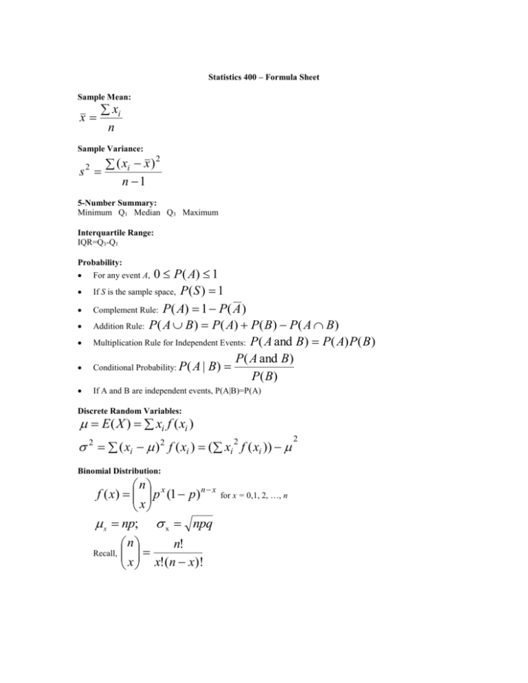
Statistics 400 – Formula Sheet
Sample Mean:
x
 xi
n
Sample Variance:
2
 ( xi  x )
s 
n 1
2
5-Number Summary:
Minimum Q1 Median Q3 Maximum
Interquartile Range:
IQR=Q3-Q1
Probability:







0  P ( A)  1
If S is the sample space, P ( S )  1
Complement Rule: P( A)  1  P( A )
Addition Rule: P ( A  B )  P ( A)  P ( B )  P ( A  B )
Multiplication Rule for Independent Events: P ( A and B )  P ( A) P ( B )
P( A and B)
Conditional Probability: P ( A | B ) 
P( B)
For any event A,
If A and B are independent events, P(A|B)=P(A)
Discrete Random Variables:
  E( X )   xi f ( xi )
 2   ( xi   ) 2 f ( xi )  ( xi 2 f ( xi ))  
Binomial Distribution:
 n
f ( x)    p x (1  p) n  x
 x
 x  np;  x  npq
 n
n!
Recall,   
 x  x!(n  x)!
 
for x = 0,1, 2, …, n
2
Z-Transformation:
Z
x

Inference for the Population Mean:
 Sample Size for a desired Margin of Error, d, for samples from a normal population:
2
 z / 2 
n



d


Large Sample Confidence Intervals

 x  z / 2

 x  z / 2
 
when  is known

n
s 
when  is unknown
n 
Small Sample Confidence Intervals
s 

x

t

/
2

n 

Independent Sample Confidence Intervals

1 1
(
x

x
)

t
s
 
 1
2
 /2 p
n
n2 
1

Inference for the Population Proportions:

Large Sample Confidence Interval for a Proportion: (use p=q=.5 for conservative CI)

 pˆ  z / 2


Large Sample Test Statistic for a Proportion:
Z

pq 

n 
pˆ  p0
p0 q0 / n
Small Sample Test Statistic for a Proportion: X = number of successes. If H0 is true, X has a binomial
distribution with parameters p0 and n.
2

Sample Size for Desired Margin of Error m:
 z*  *
n    p (1  p * )
d
T-statistics:



 x  0 
t 

s
/
n




 x1  x2
Two Sample t-statistic: t 

1 1
 sp


n
n2
1

One-Sample t-statistic:
Pooled sample variance:
df=n-1



df=n1+n2-2




 (n1  1) s12  (n2  1) s22 
2

s p  

n1  n2  2


Correlation and Regression:
Correlation:
r
1  xi  x  yi  y 


n  sx  s y 
Linear Regression Model:
yi  0  1xi   i
Parameter Estimators:
̂1  r
sy
sx
,
where
 i is N 0, 
ˆ0  y  ˆ1 x
ei  yi  yˆ i = observed y – predicted y
Residuals:
Estimate of
:
e
2
i
s  MSE 
A Level C confidence Interval for
s
where SE b1 
 x
 1 is given by:
ˆ1  t *SE ( ˆ1 )
*
 x
2
i
n2
and t is the value for the
t n  2 density curve with area C
between  t and t .
*
*
H 0 : 1  10 ,
ˆ1  10
the test statistic is t 
which has a t n  2 distribution under
SE ( ˆ1 )
t Test for
1
To test
H0
1
Standard error of the intercept
1
x2
ˆ
 0 : SE (  0 )  s 
n  xi  x 2
H 0 :  0   00 ,
ˆ0   00
the test statistic is t 
SE ( ˆ0 )
T-Test for
0
To test
1
which has a
t n  2 distribution under H 0
Estimated Mean Response
ˆ y  ˆ0  ˆ1 x *
A Level C Confidence Interval for the Mean Response is given by:
where
1 ( x*  x ) 2
SE ( ˆ y )  s

n  xi  x 2
ˆ0  ˆ1 x *  t * SE ( ˆ y )
*
and t is the value for the
t n  2 density curve
with area C between  t and t .
*
*
Predicted Value of the Response Variable
yˆ  ˆ0  ˆ1 x*
A Level C Prediction Interval for an Individual Response is given by:
where
1 ( x*  x ) 2
SE ( yˆ )  s 1  
n   xi  x 2
ˆ0  ˆ1 x*  t * SE( yˆ )
and t* is the value for the
t n  2 density curve
with area C between  t and t .
*
*
Chi-Square Tests:
Test of Independence
Independence Hypothesis
H 0 : There is no relationship between the row variable and the column
variable.
Expected Cell Counts
Test Statistic
2  
E  expected 
row total  column tot al
Overall total
(observed  expected ) 2
expected
which has the
2
distribution with (r  1)(c  1) degrees of freedom under.