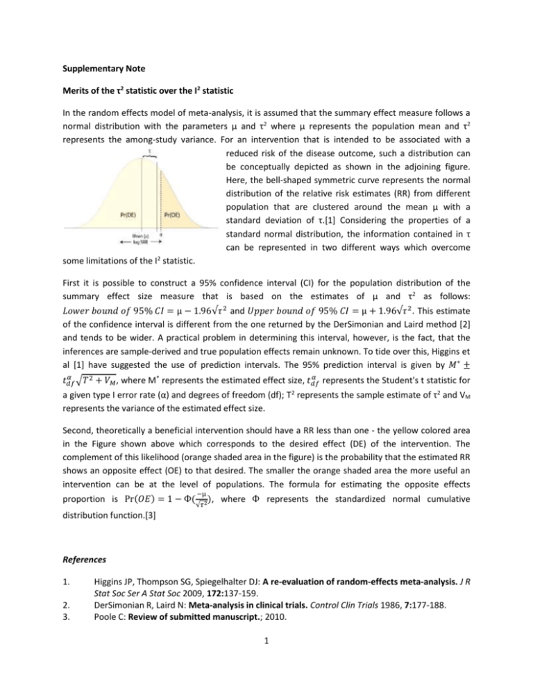
Supplementary Note
Merits of the τ2 statistic over the I2 statistic
In the random effects model of meta-analysis, it is assumed that the summary effect measure follows a
normal distribution with the parameters µ and τ2 where µ represents the population mean and τ2
represents the among-study variance. For an intervention that is intended to be associated with a
reduced risk of the disease outcome, such a distribution can
be conceptually depicted as shown in the adjoining figure.
Here, the bell-shaped symmetric curve represents the normal
distribution of the relative risk estimates (RR) from different
population that are clustered around the mean µ with a
standard deviation of τ.[1] Considering the properties of a
standard normal distribution, the information contained in τ
can be represented in two different ways which overcome
2
some limitations of the I statistic.
First it is possible to construct a 95% confidence interval (CI) for the population distribution of the
summary effect size measure that is based on the estimates of µ and τ2 as follows:
𝐿𝑜𝑤𝑒𝑟 𝑏𝑜𝑢𝑛𝑑 𝑜𝑓 95% 𝐶𝐼 = µ − 1.96√𝜏 2 and 𝑈𝑝𝑝𝑒𝑟 𝑏𝑜𝑢𝑛𝑑 𝑜𝑓 95% 𝐶𝐼 = µ + 1.96√𝜏 2. This estimate
of the confidence interval is different from the one returned by the DerSimonian and Laird method [2]
and tends to be wider. A practical problem in determining this interval, however, is the fact, that the
inferences are sample-derived and true population effects remain unknown. To tide over this, Higgins et
al [1] have suggested the use of prediction intervals. The 95% prediction interval is given by 𝑀∗ ±
𝛼
𝛼
𝑡𝑑𝑓
√𝑇 2 + 𝑉𝑀 , where M* represents the estimated effect size, 𝑡𝑑𝑓
represents the Student's t statistic for
a given type I error rate (α) and degrees of freedom (df); T2 represents the sample estimate of τ2 and VM
represents the variance of the estimated effect size.
Second, theoretically a beneficial intervention should have a RR less than one - the yellow colored area
in the Figure shown above which corresponds to the desired effect (DE) of the intervention. The
complement of this likelihood (orange shaded area in the figure) is the probability that the estimated RR
shows an opposite effect (OE) to that desired. The smaller the orange shaded area the more useful an
intervention can be at the level of populations. The formula for estimating the opposite effects
proportion is Pr(𝑂𝐸) = 1 − Ф(
−µ
√𝜏2
), where Ф represents the standardized normal cumulative
distribution function.[3]
References
1.
2.
3.
Higgins JP, Thompson SG, Spiegelhalter DJ: A re-evaluation of random-effects meta-analysis. J R
Stat Soc Ser A Stat Soc 2009, 172:137-159.
DerSimonian R, Laird N: Meta-analysis in clinical trials. Control Clin Trials 1986, 7:177-188.
Poole C: Review of submitted manuscript.; 2010.
1
2