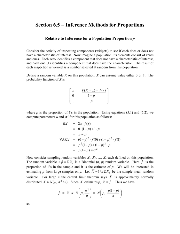
Section 6.5 − Inference Methods for Proportions
Relative to Inference for a Population Proportion p
Consider the activity of inspecting components (widgets) to see if each does or does not
have a characteristic of interest. Now imagine a population. Its elements consist of zeros
and ones. Each zero identifies a component that does not have a characteristic of interest,
and each one (1) identifies a component that does have the characteristic. The result of
each inspection is viewed as a number selected at random from this population.
Define a random variable X on this population. X can assume value either 0 or 1. The
probability function of X is
x
0

 1
P ( X = x) = f ( x) 

1− p


p
where p is the proportion of 1's in the population. Using equations (5.1) and (5.2), we
compute parameters µ and σ 2 for this population as follows:
EX
VARX
= Σx ⋅ f ( x )
= 0 ⋅ (1 − p ) + 1 ⋅ p
= p≡µ
= (0 − p) 2 ⋅ f (0) + (1 − p ) 2 ⋅ f (1)
= p 2 (1 − p ) + (1 − p) 2 ⋅ p
= p(1 − p ) ≡ σ 2
Now consider sampling random variables X1, X2, …, Xn each defined on this population.
The random variable n pˆ = Σ X i is a Binomial (n, p) random variable. Here p̂ is the
proportion of 1’s in the sample and it is the estimate of p. We will be interested in
estimating p from large samples only. Let X = 1 / n Σ X i be the sample mean random
variable. For large n the central limit theorem says X is approximately normally
distributed X ≈ N ( µ , σ 2 / n) . Since X estimates p, X ≡ pˆ . Thus we have
 σ2
pˆ ≡ X ≈ N  µ ,
n

so

 ≡ N  p, p(1 − p) 

n



Z =
pˆ − p
p (1 − p )
n
≈ N (0, 1) .
Since we do not know σ this is not useful in practice. However when we use
σˆ = pˆ (1 − pˆ ) then we have the practically useful (we are saying we know σ is σˆ )
Z =
pˆ − p
≈ N (0, 1) .
pˆ (1 − pˆ )
n
(Recall we are assuming large n.) Using this result we can make inferences (confidence
intervals and significance tests) about the parameter p using the random sample estimator
pˆ = 1 / n Σ X i .
SINGLE SAMPLE CASE
For Large n (5 ≤ n p ≤ n − 5)
Z =
pˆ − p
p (1 − p )
n
≈ N (0, 1)
(1)
and (using p̂ in place of p)
Z =
pˆ − p
≈ N (0, 1)
pˆ (1 − pˆ )
n
Using (2) an approximate 100(1 − α)% C.I. for p is
pˆ (1 − pˆ )
.
n
pˆ ± zα / 2
To test:
H 0 : p = # vs. H a : p ≠ #
the test statistic is (using (1))
Z =
pˆ − #
# (1 − # )
n
Examples 16 and 17 in Section 6.5 illustrates this.
2
(2)
TWO SAMPLE CASE
For Large n1 and n2
Z =
pˆ 1 − pˆ 2 − ( p1 − p 2 )
p1 (1 − p1 )
p (1 − p 2 )
+ 2
n1
n2
≈ N (0, 1)
(3)
and
Z =
pˆ 1 − pˆ 2 − ( p1 − p 2 )
≈ N (0, 1)
pˆ 1 (1 − pˆ 1 )
pˆ 2 (1 − pˆ 2 )
+
n1
n2
(4)
using (4) a 100(1 − α)% C.I. for p1 – p2 is (its approximate)
pˆ 1 (1 − pˆ 1 )
pˆ (1 − pˆ 2 )
+ 2
n1
n2
pˆ 1 − pˆ 2 ± zα / 2
To Test:
H 0 : p1 − p 2 = 0 vs. H a : p1 − p 2 ≠ 0
The test is (as always) based on assuming H0 true, i.e., p1 = p 2 ≡ p , so the test statistic is
obtained by pooling the two samples to estimate the common value p as p̂
pˆ =
n1 pˆ 1 + n2 pˆ 2
.
n1 + n2
Then in (3) substitute zero for p1 − p 2 in the numerator and p for p1 and p2 in the
denominator. This gives
Z =
pˆ 1 − pˆ 2
 1
1 

p (1 − p) 
+
n
n
2 
 1
.
Then using p̂ to estimate p gives the test statistic
Z =
pˆ 1 − pˆ 2
 1
1 

+
pˆ (1 − pˆ ) 
n
n
2 
 1
See Example 18 in Section 6.5 for an application.
3
.