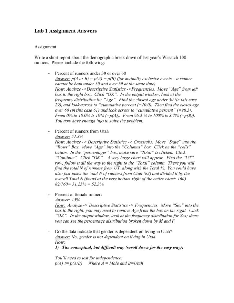
Lab 1 Assignment Answers
Assignment
Write a short report about the demographic break down of last year’s Wasatch 100
runners. Please include the following:
-
Percent of runners under 30 or over 60
Answer: p(A or B) = p(A) + p(B) (for mutually exclusive events – a runner
cannot be both under 30 and over 60 at the same time).
How: Analyze ->Descriptive Statistics ->Frequencies. Move “Age” from left
box to the right box. Click “OK”. In the output window, look at the
frequency distribution for “Age”. Find the closest age under 30 (in this case
29), and look across to “cumulative percent (=10.0). Then find the closes age
over 60 (in this case 61) and look across to “cumulative percent” (=96.3).
From 0% to 10.0% is 10% (=p(A)). From 96.3 % to 100% is 3.7% (=p(B)).
You now have enough info to solve the problem.
-
Percent of runners from Utah
Answer: 51.3%
How: Analyze -> Descriptive Statistics -> Crosstabs. Move “State” into the
“Rows” Box. Move “Age” into the “Columns” box. Click on the “cells”
button. In the “percentages” box, make sure “Total” is clicked. Click
“Continue”. Click “OK”. A very large chart will appear. Find the “UT”
row, follow it all the way to the right to the “Total” column. There you will
find the total N of runners from UT, along with the Total %. You could have
also just taken the total N of runners from Utah (82) and divided it by the
overall Total N (found at the very bottom right of the entire chart; 160).
82/160= 51.25% = 52.3%.
-
Percent of female runners
Answer: 15%
How: Analyze -> Descriptive Statistics -> Frequencies. Move “Sex” into the
box to the right; you may need to remove Age from the box on the right. Click
“OK”. In the output window, look at the frequency distribution for Sex; there
you can see the percentage distribution broken down by M and F.
-
Do the data indicate that gender is dependent on living in Utah?
Answer: No, gender is not dependent on living in Utah.
How:
1) The conceptual, but difficult way (scroll down for the easy way):
You’ll need to test for independence:
p(A) != p(A/B) Where A = Male and B=Utah
To find p(male), we can use the info we got for the previous answer (1p(female) = 1-.15 = .85). To find p(Utah) we can use information from two
answers ago (.513). To find p(male/Utah), the easiest way is to run a
crosstabs (Analyze -> Descriptive Statistics -> Crosstabs) with “State” in the
rows box, and “Sex” in the columns box. You can find p(male/Utah) this way
– just scroll down until you get to Utah, then go across to Male. This gives
you the number of males in Utah (71). To find the probability, you take the
number of males in Utah (71), divided by the total number of people in Utah
(82).
p(male) = .85, p(Utah) = .513. p(male/Utah) = (71/82 = .865)
2) The easy way
Data -> Select Cases. Click the “If Condition is Satisfied” radio button, then
click the “If” button directly below that. Move “State” into the box on the
right. Put = ‘UT’ after “State” – be sure to include the ‘ ‘ marks around
state. Click “Continue”, then “OK”. You have now essentially made SPSS do
the /Utah portion of p(male/Utah) (we are only going to be looking at Utah
when we do the analysis.
Now, Analyze -> Descriptive Statistics -> Frequencies. Move “Sex” into the
box in the right (and remove anything else that might be there. Click “OK”.
You now see the percentage of male and female given Utah. p(male = .85) !=
p(male/Utah = .866).
-
Given that a runner comes from California, what is the probability that that
runner is female?
Answer: .357
How: Data -> Select Cases. Click on the “If” button below the “If condition
is satisfied” radio button. Change the ‘UT’ to ‘CA’ (UT should still be there
from answering the last question). Click “Continue”, then click “OK”.
Analyze -> Descriptive Statistics -> Frequencies. “Sex” should already be in
the box on the right (from the last question), so just click “OK”. Now we have
the answer – we can find the proportion of females given that we’re only
looking at CA (look in the percent column).
Anything else that you find interesting…