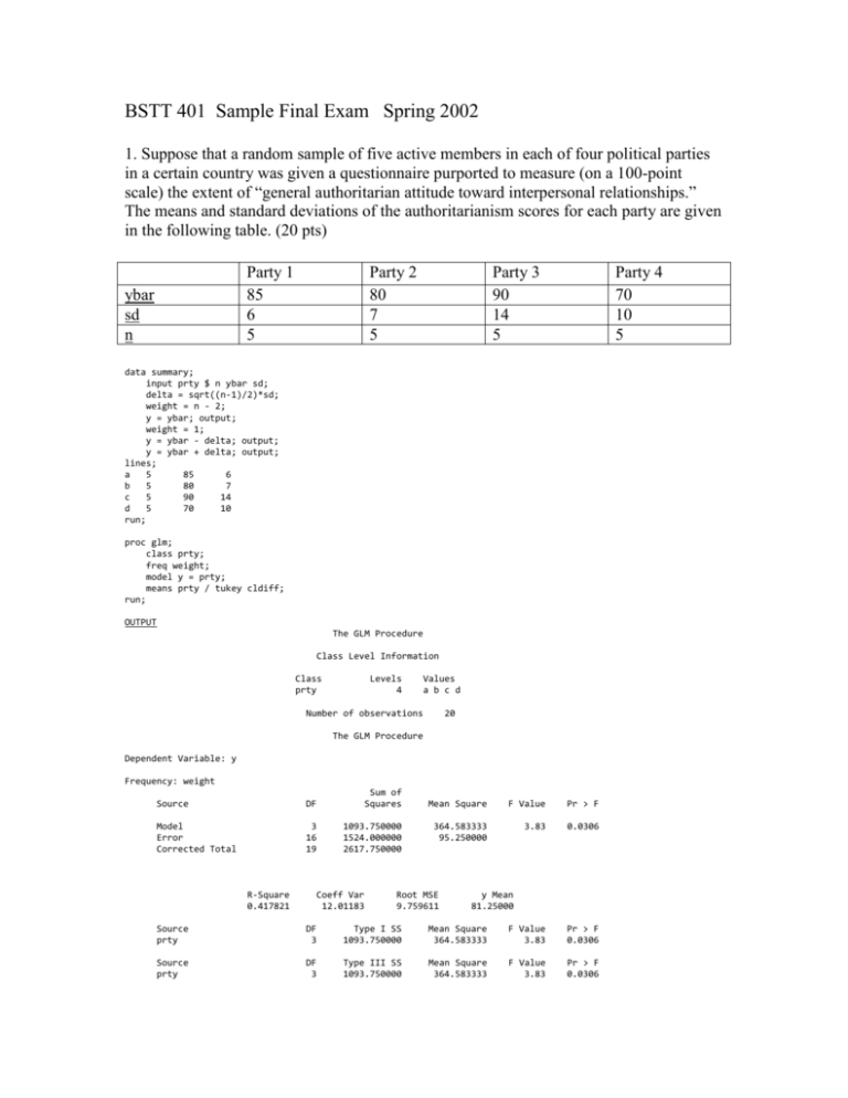
BSTT 401 Sample Final Exam Spring 2002
1. Suppose that a random sample of five active members in each of four political parties
in a certain country was given a questionnaire purported to measure (on a 100-point
scale) the extent of “general authoritarian attitude toward interpersonal relationships.”
The means and standard deviations of the authoritarianism scores for each party are given
in the following table. (20 pts)
Party 1
85
6
5
ybar
sd
n
Party 2
80
7
5
Party 3
90
14
5
Party 4
70
10
5
data summary;
input prty $ n ybar sd;
delta = sqrt((n-1)/2)*sd;
weight = n - 2;
y = ybar; output;
weight = 1;
y = ybar - delta; output;
y = ybar + delta; output;
lines;
a
5
85
6
b
5
80
7
c
5
90
14
d
5
70
10
run;
proc glm;
class prty;
freq weight;
model y = prty;
means prty / tukey cldiff;
run;
OUTPUT
The GLM Procedure
Class Level Information
Class
prty
Levels
4
Values
a b c d
Number of observations
20
The GLM Procedure
Dependent Variable: y
Frequency: weight
Source
DF
Sum of
Squares
Model
Error
Corrected Total
3
16
19
1093.750000
1524.000000
2617.750000
R-Square
0.417821
Coeff Var
12.01183
Mean Square
F Value
Pr > F
364.583333
95.250000
3.83
0.0306
Root MSE
9.759611
y Mean
81.25000
Source
prty
DF
3
Type I SS
1093.750000
Mean Square
364.583333
F Value
3.83
Pr > F
0.0306
Source
prty
DF
3
Type III SS
1093.750000
Mean Square
364.583333
F Value
3.83
Pr > F
0.0306
The GLM Procedure
Tukey's Studentized Range (HSD) Test for y
NOTE: This test controls the Type I experimentwise error rate.
Alpha
Error Degrees of Freedom
Error Mean Square
Critical Value of Studentized Range
Minimum Significant Difference
0.05
16
95.25
4.04609
17.66
Comparisons significant at the 0.05 level are indicated by ***.
prty
Comparison
c
c
c
a
a
a
b
b
b
d
d
d
-
Difference
Between
Means
a
b
d
c
b
d
c
a
d
c
a
b
5.000
10.000
20.000
-5.000
5.000
15.000
-10.000
-5.000
10.000
-20.000
-15.000
-10.000
Simultaneous 95%
Confidence Limits
-12.660
-7.660
2.340
-22.660
-12.660
-2.660
-27.660
-22.660
-7.660
-37.660
-32.660
-27.660
22.660
27.660
37.660
12.660
22.660
32.660
7.660
12.660
27.660
-2.340
2.660
7.660
***
***
a. State the model for the experiment, using dummy variables.
b. State the hypotheses.
c. Test to see where significant differences exist among parties with
respect to mean authoritarian scores.
d. Based on Tukey’s method of multiple comparisons, identify the pairs in which the
means significantly differ from one another. (Use alpha = .05)
2. The diameters (Y) of three species of pine trees (A) were compared at each of four
locations (B), using samples of three trees per species at each location. Here A is
considered fixed and B, random. The resulting data are given in the data in the following
SAS program. (15 pts)
data mixed;
input A B @@;
do i = 1 to 3;
input yield @@;
output;
end;
drop i;
cards;
1
1
1
1
2
2
2
2
3
3
3
3
;
1
2
3
4
1
2
3
4
1
2
3
4
15.71
16.21
17.32
17.54
17.83
17.68
17.95
18.08
14.78
15.80
16.21
16.99
16.02
16.36
17.03
17.82
17.45
17.70
18.01
18.56
15.03
15.62
16.44
16.39
15.90
16.33
17.22
17.62
16.96
17.52
18.41
18.90
14.63
15.77
16.32
17.02
proc glm;
Title ‘when A is fixed and B is random’;
class A B;
model yield = A B A*B;
random B A*B/test;
run;
Output
WHEN A IS FIXED AND B IS RANDOM
The GLM Procedure
Class Level Information
Class
A
B
Levels
Values
3
1 2 3
4
1 2 3 4
Number of observations
36
The GLM Procedure
Dependent Variable: yield
Source
DF
Sum of
Squares
Model
Error
Corrected Total
11
24
35
39.06083056
1.39026667
40.45109722
R-Square
0.965631
Coeff Var
1.427132
Mean Square
F Value
Pr > F
3.55098460
0.05792778
61.30
<.0001
Root MSE
0.240682
yield Mean
16.86472
Source
A
B
A*B
DF
2
3
6
Type I SS
24.31027222
13.81794167
0.93261667
Mean Square
12.15513611
4.60598056
0.15543611
F Value
209.83
79.51
2.68
Pr > F
<.0001
<.0001
0.0389
Source
A
B
A*B
DF
2
3
6
Type III SS
24.31027222
13.81794167
0.93261667
Mean Square
12.15513611
4.60598056
0.15543611
F Value
209.83
79.51
2.68
Pr > F
<.0001
<.0001
0.0389
The GLM Procedure
Source
A
B
A*B
Type III Expected Mean Square
Var(Error) + 3 Var(A*B) + Q(A)
Var(Error) + 3 Var(A*B) + 9 Var(B)
Var(Error) + 3 Var(A*B)
The GLM Procedure
Tests of Hypotheses for Mixed Model Analysis of Variance
Dependent Variable: yield
Source
DF
Type III SS
Mean Square
F Value
Pr > F
2
3
6
24.310272
13.817942
0.932617
12.155136
4.605981
0.155436
78.20
29.63
<.0001
0.0005
Source
DF
Type III SS
Mean Square
F Value
Pr > F
A*B
Error: MS(Error)
6
24
0.932617
1.390267
0.155436
0.057928
2.68
0.0389
A
B
Error: MS(A*B)
a. State the model
b. State the three possible hypotheses.
c. Test to see where significant differences exist among species, locations as well as the
interactions with respect to mean diameters of the trees.
3. 11 students were asked about their attitude toward biostatistics before and after taking
BSTT401. (10 pts)
BSTT 401
Column totals
Before
After
Opinion about biostatistics
Like
Dislike
2
9
7
4
9
13
Row totals
11
11
22
Here the problem is that the number of students who answered the question is not 22 but
11. Each student answered the question twice before and after taking BSTT401.
Therefore, each observation is not independent. Three students said that they disliked the
biostatistics before and after taking the class.
a. Construct a table about the pairs of responses.
After
Like
Before
Like
Dislike
Column totals
Row totals
Dislike
b. Calculate McNemar’s Test Statistics and see whether their attitude toward biostatistics
significantly changed or not. (refer to the fact that the critical value of X 2 with one
degree of freedom at  =.05 is 3.841).
4. Suppose we want to find out the relationship between lung cancer and BMI and the
following data have been collected. (20 pts)
BMI
Above 30 (Obese)
25 – 30 (Overweight)
Below 25 (Normal)
Heart attacks
Yes
20
10
5
SAS program
Data cancer;
input bmi $ attack $ wt;
if bmi= ‘obese’
then X1 = 1; else X1=0;
if bmi= ‘overwt’
then X2 = 1; else X2 = 0;
if attack = ‘yes’
then Y = 1 ;
else Y = 0;
lines;
obese
yes 25
obese
no
5
overwt yes 10
overwt no
20
normal yes
5
normal no
25
run;
proc logistic descending;
weight wt;
model Y = X1 X2 /link=logit;
run;
Output
The LOGISTIC Procedure
Model Information
No
5
20
25
Data Set
Response Variable
Number of Response Levels
Number of Observations
Weight Variable
Sum of Weights
Link Function
Optimization Technique
WORK.CANCER
Y
2
6
wt
90
Logit
Fisher's scoring
Response Profile
Total
Y
Frequency
1
3
0
3
Ordered
Value
1
2
Total
Weight
40.000000
50.000000
Model Convergence Status
Convergence criterion (GCONV=1E-8) satisfied.
Model Fit Statistics
Intercept
Intercept
and
Criterion
Only
Covariates
AIC
125.653
98.258
SC
125.445
97.633
-2 Log L
123.653
92.258
Testing Global Null Hypothesis: BETA=0
Test
Likelihood Ratio
Score
Wald
Chi-Square
31.3949
29.2500
23.3637
DF
2
2
2
Pr > ChiSq
<.0001
<.0001
<.0001
The LOGISTIC Procedure
Parameter
Intercept
X1
X2
Analysis of Maximum Likelihood Estimates
Standard
DF
Estimate
Error
Chi-Square
1
1
1
-1.6093
3.2186
0.9162
0.4899
0.6928
0.6245
Pr > ChiSq
10.7921
21.5842
2.1523
0.0010
<.0001
0.1424
Odds Ratio Estimates
Effect
X1
X2
Point
Estimate
95% Wald
Confidence Limits
24.994
2.500
6.429
0.735
97.170
8.500
Association of Predicted Probabilities and Observed Responses
Percent Concordant
Percent Discordant
Percent Tied
Pairs
33.3
33.3
33.3
9
Somers' D
Gamma
Tau-a
c
0.000
0.000
0.000
0.500
a) State the model.
b) Based on G 2 statistics, state whether the model is significant or not.
c) Find OR Obese vs Normal , and its confidence interval and interpret the result.
d) Find OR Overweight vs Normal and its confidence interval and interpret the result.
5. The objective of this study is to compare incidence of nonmelanoma skin cancer
among women in Minneapolis-St. Paul and Dallas-Ft. Worth. (15 pts)
SAS program
data skin1;
input agegroup $ city $ cases pop @@;
lpop = log(pop);
if agegroup='15-24' then age1=1; else age1=0;
if agegroup='25-34' then age2=1; else age2=0;
if agegroup='35-44' then age3=1; else age3=0;
if agegroup='45-54' then age4=1; else age4=0;
if agegroup='55-64' then age5=1; else age5=0;
if agegroup='65-74' then age6=1; else age6=0;
if agegroup='75-84' then age7=1; else age7=0;
if city='Dallas'
then city1=1; else city1=0;
lines;
15-24 Paul
1 172675
25-34 Paul 16 123065
35-44 Paul 30 96216
45-54 Paul 71 92051
55-64 Paul 102 72159
65-74 Paul 130 54722
75-84 Paul 133 32185
85+
Paul 40
8328
run;
15-24
25-34
35-44
45-54
55-64
65-74
75-84
85+
Dallas
Dallas
Dallas
Dallas
Dallas
Dallas
Dallas
Dallas
4
38
119
221
259
310
226
65
181343
146207
121374
111353
83004
55932
29007
7538
proc genmod;
model cases = age1 age2 age3 age4 age5 age6 age7 city1
/dist=poisson link = log
offset=lpop
/* to normalize the fitted cell
type1 type3;
run;
Output
The GENMOD Procedure
Model Information
Data Set
WORK.SKIN2
Distribution
Poisson
Link Function
Log
means */
Dependent Variable
Offset Variable
Observations Used
cases
lpop
16
Criteria For Assessing Goodness Of Fit
Criterion
DF
Value
Value/DF
Deviance
Scaled Deviance
Pearson Chi-Square
Scaled Pearson X2
Log Likelihood
Algorithm converged.
7
7
7
7
8.1950
8.1950
8.0626
8.0626
7201.8635
1.1707
1.1707
1.1518
1.1518
Using EXCEL,
the p-value for D
is .316.
Analysis Of Parameter Estimates
Parameter
DF
Estimate
Standard
Error
Intercept
age1
age2
age3
age4
age5
age6
age7
city1
Scale
1
1
1
1
1
1
1
1
1
0
-5.4797
-6.1782
-3.5480
-2.3308
-1.5830
-1.0909
-0.5328
-0.1196
0.8043
1.0000
0.1037
0.4577
0.1675
0.1275
0.1138
0.1109
0.1086
0.1109
0.0522
0.0000
Wald 95% Confidence
Limits
-5.6828
-7.0753
-3.8763
-2.5807
-1.8061
-1.3083
-0.7457
-0.3371
0.7020
1.0000
-5.2765
-5.2810
-3.2197
-2.0810
-1.3599
-0.8735
-0.3199
0.0978
0.9066
1.0000
ChiSquare
Pr > ChiSq
2794.67
182.17
448.76
334.36
193.38
96.75
24.06
1.16
237.34
<.0001
<.0001
<.0001
<.0001
<.0001
<.0001
<.0001
0.2809
<.0001
OTE: The scale parameter was held fixed.
LR Statistics For Type 1 Analysis
ChiSource
Deviance
DF
Square
Intercept
2790.3403
age1
1808.1517
1
982.19
age2
1115.2415
1
692.91
age3
708.1006
1
407.14
age4
455.6933
1
252.41
age5
306.8205
1
148.87
age6
268.0675
1
38.75
age7
266.9143
1
1.15
city1
8.1950
1
258.72
Pr > ChiSq
<.0001
<.0001
<.0001
<.0001
<.0001
<.0001
0.2829
<.0001
LR Statistics For Type 3 Analysis
ChiSource
DF
Square
Pr > ChiSq
age1
1
626.74
<.0001
age2
1
418.90
<.0001
age3
1
252.07
<.0001
age4
1
145.04
<.0001
age5
1
78.00
<.0001
age6
1
21.50
<.0001
age7
1
1.14
0.2862
city1
1
258.72
<.0001
a) State the model
b) Based on D statistics, state whether the model fits the data well or not.
c) Find RR Dallas vs Paul and interpret the result.
6. From the same context with Problems 1 & 2, subjects 1-8 came from Clinic A,
subjects 9 –15, from Clinic B, and subjects 16-20 from Clinic C were added
later. (10 pts)
Subject
1
2
3
4
5
6
7
8
Clinic A
1.69
2.22
3.07
3.35
3.00
2.74
3.61
5.14
Subject
9
10
11
12
13
14
15
Clinic B
2.44
4.17
2.42
2.94
3.04
4.62
4.42
Subject
16
17
18
19
20
title1 'Nonparametric problem 3';
data one;
input subject before after @@;
if subject < 9 then clinic="A";
if subject > 8 and subject < 16 then clinic="B";
if subject > 15 then clinic="C";
drop before;
cards;
1 1.69 1.69 9 2.58 2.44
2 2.77 2.22 10 1.84 4.17
3 1.00 3.07 11 1.89 2.42
4 1.66 3.35 12 1.91 2.94
5 3.00 3.00 13 1.75 3.04
6 0.85 2.74 14 2.46 4.62
7 1.42 3.61 15 2.35 4.42
8 2.82 5.14 16
.
2.34
17 .
3.17 18
.
4.42
19 .
4.94 20
.
5.04
;
run;
proc npar1way wilcoxon;
class clinic;
var after;
run;
Edited SAS output
The NPAR1WAY Procedure
Wilcoxon Scores (Rank Sums) for Variable after
Classified by Variable clinic
Sum of
Expected
Std Dev
Mean
clinic
N
Scores
Under H0
Under H0
Score
ƒƒƒƒƒƒƒƒƒƒƒƒƒƒƒƒƒƒƒƒƒƒƒƒƒƒƒƒƒƒƒƒƒƒƒƒƒƒƒƒƒƒƒƒƒƒƒƒƒƒƒƒƒƒƒƒƒƒƒƒƒƒƒƒƒƒƒƒƒƒ
A
8
72.00
84.00
12.956608
9.000000
B
7
71.50
73.50
12.614684
10.214286
C
5
66.50
52.50
11.452131
13.300000
Average scores were used for ties.
Kruskal-Wallis Test
Chi-Square
1.6519
Clinic C
2.34
3.17
4.42
4.94
5.04
DF
Pr > Chi-Square
2
0.4378
Can one conclude that the FEV levels from these three groups are different? Let
  0.05 and find the p-value.
7. Assume that the following table came from the analysis of a randomized-blocks
design ANOVA. (10 pts)
Source
Treatments
df
4
SS
b
MS
e
F
5.00
Blocks
a
c
48.00
6.00
Error
20
d
f
Show your work on how you got the answers for a) – f).