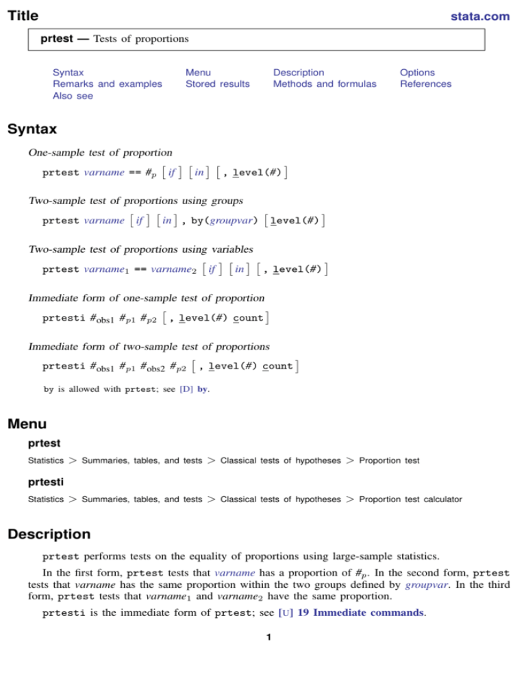
Title
stata.com
prtest — Tests of proportions
Syntax
Remarks and examples
Also see
Menu
Stored results
Description
Methods and formulas
Options
References
Syntax
One-sample test of proportion
prtest varname == #p if
in
, level(#)
Two-sample test of proportions using groups
prtest varname if
in , by(groupvar) level(#)
Two-sample test of proportions using variables
prtest varname1 == varname2 if
in
, level(#)
Immediate form of one-sample test of proportion
prtesti # obs1 # p1 # p2 , level(#) count
Immediate form of two-sample test of proportions
prtesti # obs1 # p1 # obs2 # p2 , level(#) count
by is allowed with prtest; see [D] by.
Menu
prtest
Statistics
>
Summaries, tables, and tests
>
Classical tests of hypotheses
>
Proportion test
>
Summaries, tables, and tests
>
Classical tests of hypotheses
>
Proportion test calculator
prtesti
Statistics
Description
prtest performs tests on the equality of proportions using large-sample statistics.
In the first form, prtest tests that varname has a proportion of #p . In the second form, prtest
tests that varname has the same proportion within the two groups defined by groupvar. In the third
form, prtest tests that varname1 and varname2 have the same proportion.
prtesti is the immediate form of prtest; see [U] 19 Immediate commands.
1
2
prtest — Tests of proportions
The bitest command is a better version of the first form of prtest in that it gives exact p-values.
Researchers should use bitest when possible, especially for small samples; see [R] bitest.
Options
Main
by(groupvar) specifies a numeric variable that contains the group information for a given observation.
This variable must have only two values. Do not confuse the by() option with the by prefix; both
may be specified.
level(#) specifies the confidence level, as a percentage, for confidence intervals. The default is
level(95) or as set by set level; see [U] 20.7 Specifying the width of confidence intervals.
count specifies that integer counts instead of proportions be used in the immediate forms of prtest.
In the first syntax, prtesti expects that #obs1 and #p1 are counts—#p1 ≤ #obs1 —and #p2 is a
proportion. In the second syntax, prtesti expects that all four numbers are integer counts, that
#obs1 ≥ #p1 , and that #obs2 ≥ #p2 .
Remarks and examples
stata.com
The prtest output follows the output of ttest in providing a lot of information. Each proportion
is presented along with a confidence interval. The appropriate one- or two-sample test is performed,
and the two-sided and both one-sided results are included at the bottom of the output. For a two-sample
test, the calculated difference is also presented with its confidence interval. This command may be
used for both large-sample testing and large-sample interval estimation.
Example 1: One-sample test of proportion
In the first form, prtest tests whether the mean of the sample is equal to a known constant. Assume
that we have a sample of 74 automobiles. We wish to test whether the proportion of automobiles that
are foreign is different from 40%.
. use http://www.stata-press.com/data/r13/auto
(1978 Automobile Data)
. prtest foreign == .4
One-sample test of proportion
foreign: Number of obs =
Variable
Mean
foreign
.2972973
74
Std. Err.
[95% Conf. Interval]
.0531331
.1931583
p = proportion(foreign)
Ho: p = 0.4
Ha: p < 0.4
Ha: p != 0.4
Pr(Z < z) = 0.0357
Pr(|Z| > |z|) = 0.0713
.4014363
z =
-1.8034
Ha: p > 0.4
Pr(Z > z) = 0.9643
The test indicates that we cannot reject the hypothesis that the proportion of foreign automobiles is
0.40 at the 5% significance level.
prtest — Tests of proportions
3
Example 2: Two-sample test of proportions
We have two headache remedies that we give to patients. Each remedy’s effect is recorded as 0
for failing to relieve the headache and 1 for relieving the headache. We wish to test the equality of
the proportion of people relieved by the two treatments.
. use http://www.stata-press.com/data/r13/cure
. prtest cure1 == cure2
Two-sample test of proportions
cure1: Number of obs =
cure2: Number of obs =
Variable
Mean
Std. Err.
cure1
cure2
.52
.7118644
.0706541
.0589618
diff
-.1918644
under Ho:
.0920245
.0931155
z
-2.06
P>|z|
[95% Conf. Interval]
.3815205
.5963013
.6584795
.8274275
-.372229
-.0114998
0.039
diff = prop(cure1) - prop(cure2)
Ho: diff = 0
Ha: diff < 0
Pr(Z < z) = 0.0197
50
59
z =
Ha: diff != 0
Pr(|Z| < |z|) = 0.0394
-2.0605
Ha: diff > 0
Pr(Z > z) = 0.9803
We find that the proportions are statistically different from each other at any level greater than 3.9%.
Example 3: Immediate form of one-sample test of proportion
prtesti is like prtest, except that you specify summary statistics rather than variables as
arguments. For instance, we are reading an article that reports the proportion of registered voters
among 50 randomly selected eligible voters as 0.52. We wish to test whether the proportion is 0.7:
. prtesti 50 .52 .70
One-sample test of proportion
x: Number of obs =
50
Variable
Mean
Std. Err.
[95% Conf. Interval]
x
.52
.0706541
.3815205
p = proportion(x)
Ho: p = 0.7
Ha: p < 0.7
Pr(Z < z) = 0.0027
z =
Ha: p != 0.7
Pr(|Z| > |z|) = 0.0055
.6584795
-2.7775
Ha: p > 0.7
Pr(Z > z) = 0.9973
Example 4: Immediate form of two-sample test of proportions
To judge teacher effectiveness, we wish to test whether the same proportion of people from
two classes will answer an advanced question correctly. In the first classroom of 30 students, 40%
answered the question correctly, whereas in the second classroom of 45 students, 67% answered the
question correctly.
4
prtest — Tests of proportions
. prtesti 30 .4 45 .67
Two-sample test of proportions
x: Number of obs =
y: Number of obs =
Variable
Mean
Std. Err.
x
y
.4
.67
.0894427
.0700952
diff
-.27
under Ho:
.1136368
.1169416
z
P>|z|
-2.31
[95% Conf. Interval]
.2246955
.532616
.5753045
.807384
-.4927241
-.0472759
0.021
diff = prop(x) - prop(y)
Ho: diff = 0
Ha: diff < 0
Pr(Z < z) = 0.0105
30
45
z =
Ha: diff != 0
Pr(|Z| < |z|) = 0.0210
-2.3088
Ha: diff > 0
Pr(Z > z) = 0.9895
Stored results
prtest and prtesti store the following in r():
Scalars
r(z)
z statistic
r(P #) proportion for variable #
r(N #) number of observations for variable #
Methods and formulas
See Acock (2014, 155–161) for additional examples of tests of proportions using Stata.
A large-sample 100(1 − α)% confidence interval for a proportion p is
r
pb ± z1−α/2
pb qb
n
and a 100(1 − α)% confidence interval for the difference of two proportions is given by
s
(b
p1 − pb2 ) ± z1−α/2
pb1 qb1
pb2 qb2
+
n1
n2
where qb = 1 − pb and z is calculated from the inverse cumulative standard normal distribution.
The one-tailed and two-tailed tests of a population proportion use a normally distributed test
statistic calculated as
pb − p0
z=p
p0 q0 /n
where p0 is the hypothesized proportion. A test of the difference of two proportions also uses a
normally distributed test statistic calculated as
prtest — Tests of proportions
z=p
5
pb1 − pb2
pbp qbp (1/n1 + 1/n2 )
where
pbp =
x1 + x2
n1 + n2
and x1 and x2 are the total number of successes in the two populations.
References
Acock, A. C. 2014. A Gentle Introduction to Stata. 4th ed. College Station, TX: Stata Press.
Wang, D. 2000. sg154: Confidence intervals for the ratio of two binomial proportions by Koopman’s method. Stata
Technical Bulletin 58: 16–19. Reprinted in Stata Technical Bulletin Reprints, vol. 10, pp. 244–247. College Station,
TX: Stata Press.
Also see
[R] bitest — Binomial probability test
[R] proportion — Estimate proportions
[R] ttest — t tests (mean-comparison tests)
[MV] hotelling — Hotelling’s T-squared generalized means test