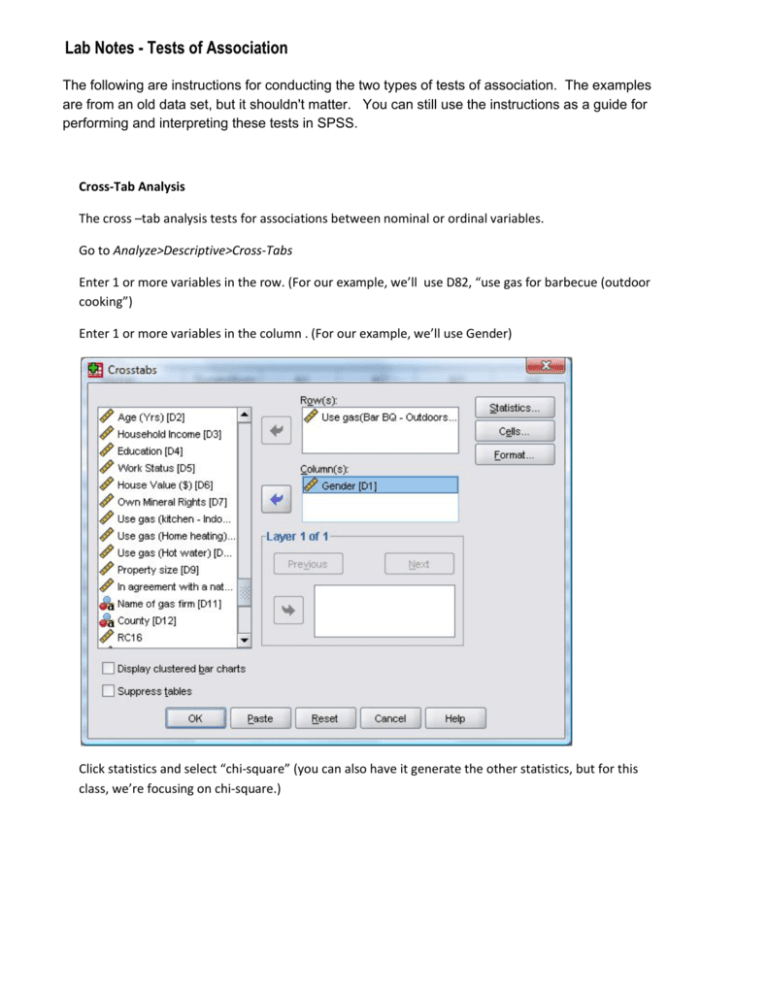
Lab Notes - Tests of Association
The following are instructions for conducting the two types of tests of association. The examples
are from an old data set, but it shouldn't matter. You can still use the instructions as a guide for
performing and interpreting these tests in SPSS.
Cross-Tab Analysis
The cross –tab analysis tests for associations between nominal or ordinal variables.
Go to Analyze>Descriptive>Cross-Tabs
Enter 1 or more variables in the row. (For our example, we’ll use D82, “use gas for barbecue (outdoor
cooking”)
Enter 1 or more variables in the column . (For our example, we’ll use Gender)
Click statistics and select “chi-square” (you can also have it generate the other statistics, but for this
class, we’re focusing on chi-square.)
Click “cells”, check “row”, “column” and “total” under Percentages
You’ll get the following output.
D82 Use gas(Bar BQ - Outdoors) * D1 Gender Crosstabulation
D1 Gender
1 Male
D82 Use gas(Bar BQ -
0 Don't use gas
Count
Outdoors)
411
825
50.2%
49.8%
100.0%
% within D1 Gender
46.2%
51.9%
48.8%
% of Total
24.5%
24.3%
48.8%
483
381
864
55.9%
44.1%
100.0%
% within D1 Gender
53.8%
48.1%
51.2%
% of Total
28.6%
22.6%
51.2%
897
792
1689
53.1%
46.9%
100.0%
100.0%
100.0%
100.0%
53.1%
46.9%
100.0%
BQ - Outdoors)
Count
% within D82 Use gas(Bar
BQ - Outdoors)
Total
Total
414
% within D82 Use gas(Bar
1 Use gas
2 Female
Count
% within D82 Use gas(Bar
BQ - Outdoors)
% within D1 Gender
% of Total
Chi-Square Tests
Value
Pearson Chi-Square
Continuity Correction
Likelihood Ratio
Exact Sig. (2-
Exact Sig. (1-
sided)
sided)
sided)
a
1
.019
5.319
1
.021
5.549
1
.018
5.546
b
df
Asymp. Sig. (2-
Fisher's Exact Test
.019
Linear-by-Linear Association
5.543
N of Valid Cases
1689
1
.019
a. 0 cells (.0%) have expected count less than 5. The minimum expected count is 386.86.
b. Computed only for a 2x2 table
.011
The first statistic you should look at is the significance of the chi-square. Since the significance level is
.019, which is <.05, we can reject the null hypothesis of no relationship. There does appear to be a
relationship between gender and outdoor cooking.
The chi-square test doesn’t provide us with any statistical measure of direction or strength, so we have
to look at the table. Approximately 54% of men cook outdoors with gas, while only 48% of men do. So
there appears to be a positive relationship between being male and cooking outdoors. You could also
read the table in the other direction, and say that of those who cook outdoors with gas, 56% are male
and 44% are female.
Pearson’s Test of Bivariate Correlation
But what if we want to test for correlations between continuous measures (ratio or interval)?
Go to Analyze>Correlate>Bivariate Correlations
Select the two (or more) variables you’re interested in and double click them. For our example, we’ll
use financial gain (FINGAIN) and materialism (MATERIAL).
Be sure that you select “Pearson” under correlation coefficients, “Two-tailed” under test of sginficance
and check the option to “Flag significant correlations”.
Click OK, and you’ll get the output below.
Correlations
MATERIAL Materialism
Pearson Correlation
MATERIAL
FINGAIN
Materialism
Financial Gain
1.000
Sig. (2-tailed)
FINGAIN Financial Gain
.211
**
.000
N
1676
1674
Pearson Correlation
.211
**
1.000
Sig. (2-tailed)
.000
N
1674
1676
**. Correlation is significant at the 0.01 level (2-tailed).
To check for correlations, first look for the presence, using the significance statistic. In this case, the level
of significance is .000, which is less than .05 so it is significant. We can reject the null hypothesis that
there is no relationship between materialism and financial gain.
Next, we check for strength and direction. The Pearson correlation of .211 is on the lower end of the 0-1
scale, but for social science research, it is fairly strong. For direction, look at the sign of the correlation
coefficient. It is positive, so the relationship is positive. Higher levels of materialism are associated with
higher levels of desire for financial gain.