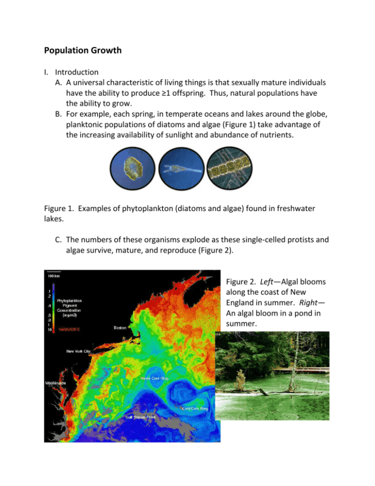
Population Growth
I. Introduction
A. A universal characteristic of living things is that sexually mature individuals
have the ability to produce ≥1 offspring. Thus, natural populations have
the ability to grow.
B. For example, each spring, in temperate oceans and lakes around the globe,
planktonic populations of diatoms and algae (Figure 1) take advantage of
the increasing availability of sunlight and abundance of nutrients.
Figure 1. Examples of phytoplankton (diatoms and algae) found in freshwater
lakes.
C. The numbers of these organisms explode as these single-celled protists and
algae survive, mature, and reproduce (Figure 2).
Figure 2. Left—Algal blooms
along the coast of New
England in summer. Right—
An algal bloom in a pond in
summer.
2
D. Populations of zooplankton (Figure 3) respond to the “spring blooms” of
diatoms by increasing their own numbers dramatically.
Figure 3. Examples of zooplankton found in freshwater lakes. Zooplankton feed
on phytoplankton.
E. Sizes of populations fluctuate in terrestrial, as well as aquatic,
environments.
F. The capacity for population growth, even among vertebrates, is enormous,
a fact that is sometimes clearly demonstrated when species are introduced
to new regions having suitable habitat. Four examples follow.
1. In 1937, 2 male and 6 female ring-necked pheasants (Phasianus
colchicus) were released on Protection Island, Washington, increased to
1,325 adults within 5 years, a 166-fold increase (Einarsen 1945).
2. When domestic sheep were introduced into Tasmania, a large island off
the southeastern coast of Australia, the population increased from
fewer than 200,000 in 1820 to more than 2 million by 1850.
3. In 1977, 8 tule elk were introduced to the Grizzly Island Wildlife Area
northeast of San Francisco. By 1986, the population had increased to
150 animals (Gogan and Barrett 1988).
4. Perhaps the most meaningful and dramatic example of the capacity of
natural populations to grow is that of our own species.
a. Although humans are not the most numerous animal species on
Earth, the proliferation of the human species is, by any accounting, a
remarkable ecological event.
b. The human population began to expand rapidly after 1600, reaching
1 billion by the early 1800s, doubling that number by 1930, and
doubling again by 1975. In 1995, the global human population
reached 6 billion. There are currently 7.3 billion people alive on
Earth today.
3
G. Ever since humans began to understand the consequences of the rapid
increase in its numbers, human population growth has been a cause for
economic and ecological concern.
1. These concerns led to the development of mathematical techniques to
predict the growth of populations and to intensive study of natural and
laboratory populations to learn about mechanisms of population growth
and regulation.
2. As a result, we now have a general understanding of the causes of
fluctuations in natural populations and the effects of crowding on birth
and death rates.
3. In this section, we will examine the factors that determine rates and
patterns of population growth.
II. Some basic principles of population growth
A. At its simplest, studying and managing a wildlife population is really nothing
more than keeping track of the 4 components of population change: births,
deaths, immigration, and emigration.
B. Population growth is accomplished principally by reproduction, although
populations may also increase in size by immigration (and may decrease in
size by emigration and death).
C. Mathematically:
Nt+1 = Nt + Bt - dt + It - Et,
Equation 1
where:
Nt+1 = population size at time t+1 ;
Nt = population size at time t ;
B = births;
D = deaths;
I = immigrants;
E = emigrants.
D. If you were managing a business, you would be interested in knowing how
much money was being paid out of the business, relative to how much
money was coming in. The net difference represents your profit. The same
is true for managing a wildlife population. By knowing the net change in
the size of the wildlife population from 1 year to the next, you as a wildlife
4
manager know whether the population is profitable (i.e., gaining in size), or
headed towards bankruptcy (i.e., becoming smaller).
E. Individuals may be added to populations by reproducing continuously or
reproducing during discrete reproductive seasons.
1. For example, when young are added to the population only at specific
times of the year, during discrete reproductive periods, the population is
said to have geometric growth, in which the increment of increase in
population size is proportional to the number of individuals in the
population at the beginning of the breeding season.
2. However, there are some organisms—humans are a good example—
that have no distinct reproductive season, but instead add young at any
time of the year. Such populations are augmented more or less
continuously. This pattern of growth, referred to as exponential
growth, is the one we shall take up first.
III. Unlimited population growth: exponential growth.
A. A population growing exponentially increases according to the equation:
Nt = Noert,
Equation 2
where:
Nt = the number of individuals in the population after t units of time;
No = the initial population size (t = 0);
r = the exponential growth rate;
t = time unit (usually in years);
e = the base of the natural logarithms (2.72)
B. Exponential growth results in a continuous curve of increase (or decrease,
when the rt term is negative) whose slope varies in direct relation to the
size of the population.
C. The term er is the factor by which the population increases during each
time unit, often written as the lowercase Greek lambda ( λ ). That is, when t
= 1, Nt = Noer, or Nt = No λ .
D. To illustrate the use of this equation let's say that the elk population in
Arkansas has a population growth rate of r = 0.013. In 2011, the population
was estimated to be 500. What will the population be in 2020?
5
The elapsed time (t) will be 2020-2011 = 9 years.
Nt = Noert
= 500 x e(0.013 x 9)
=
E. Rate of exponential population increase.
1. The rate of increase of a population undergoing exponential growth at a
particular instant in time—the instantaneous rate of increase—is the
differential of the exponential equation:
dN
= rN ,
dt
Equation 3
where:
dN = change in number
dt = change in time
r = the per head maximum potential growth rate
N = number of individuals in a population.
2. This equation encompasses 2 principles.
a. First, the exponential growth rate (r) expresses population increase
(or decrease) on a per individual basis.
dN
b. Second, the rate of increase (
) varies in direct proportion to the
dt
size of the population (N).
3. In other words, the differential exponential equation above could read:
(the rate of change in population size) = (the contribution of each
individual to population growth) x (the number of individuals in the
population).
4. As an example, suppose we have a population of 100 bobwhite quail (N)
and each individual has the average capability of contributing 1/4 (0.25)
of an individual to the population in a given unit of time (r). The change
dN
dN
) would be expressed as:
=
in number per unit of time (
dt
dt
0.25(100) = 25 quail.
6
E. Clarifying the 2 equations of exponential growth.
1. You have just been introduced to 2 mathematical models that help us
conceptualize how populations grow exponentially. Let’s briefly review
each one.
2. The formula by which exponential population growth is generally
dN
dN
is
represented is:
= rN. This is a differential equation in which
dt
dt
the population growth rate. It refers to the change in numbers (dN) per
time interval (dt) when this interval is very small, so that we are taking
an instantaneous reading--a quick snapshot--of rate of growth.
3. If we wish to look instead at the population size at various times during
exponential population growth, an equivalent expression is the integral
equation: Nt = Noert.
F. Exponential growth in nature
1. Some of the assumptions of the exponential growth model, such as a
constant growth rate or per capita increase, may seem a bit unrealistic,
so it is reasonable to ask whether populations in nature ever grow at an
exponential rate. The answer is a qualified yes.
2. Natural populations may grow at exponential rates for relatively short
periods of time in the presence of abundant resources.
3. Figure 4 shows the exponential growth of a colonizing population of
Scotch pine (Pinus sylvestris) in Great Britain.
Figure 4. Exponential growth of a colonizing population of Scotch pine (Pinus
sylvestris) in Britain. Figure from Molles (1999), page 212.
7
a. As the last ice age was ending, tree populations in the Northern
Hemisphere followed the retreating glaciers northward.
b. Ecologists have documented these movements by studying the
sediments of lakes, where the pollen of wind-pollinated tree species
was deposited.
c. By counting the number of pollen grains/cm2 deposited each year,
researchers have been able to reconstruct changes in tree population
densities in the surrounding landscape.
4. Figure 5 shows exponential growth of collared doves in Great Britain.
Figure 5. Exponential growth of collared doves in Britain. Figure from Molles
(1999), page 212.
G. The concept of the “r” value.
1. The exponential growth rate is a measure of the capacity of a population
for increase; it always implies numbers/time interval.
2. Some of the life history traits that influence whether r is high or low
include:
a. Number of offspring per breeding season (e.g., the number of young
in a litter and the number of litters per year);
b. Survival up to and through reproductive age;
c. Age at which reproduction begins;
8
d. Length of the reproductive age of the organism.
1) At 1 extreme are organisms such as salmon that breed only once
in their lifetime (semeloperous).
2) Many other types of organisms breed every year, or at least more
than once, until death or old age (iteroperous).
3. Looking at the geographical range of a species in terms of population
ecology, the range boundaries are approximately the line at which r = 0.
Outside the line, populations of the species, if they somehow get a start,
will decline, while inside the line, the populations will have a positive
capacity for growth.
4. In theory at least, each population has an optimal environment, with
abundant space and resources, free from predators and competitors,
and so forth, in which it’s r would attain the maximum possible value.
This value is sometimes referred to formally as rmax, the maximum
intrinsic rate of natural increase. Obviously, the realized r in the great
majority of the less-than-perfect environments, are well below rmax.
5. On average, small organisms have higher rates of per capita increase, r,
and more variable populations, while large organisms have lower rvalues and more stable populations (Figure 6).
Figure 6. The relationship between body size and r. Figure from Molles (1999),
page 219.
IV. Geometric population growth
9
A. In cases in which young are added to the population only at specific times
of the year, the exponential models may not be the best representation of
population growth.
B. Most wildlife populations restrict reproduction to a particular time of year:
the population grows during the breeding season, and then usually declines
between 1 breeding season and the next because of mortality and
emigration.
C. We can use the population of phlox studied by Leverich and Levin (1979) to
build a model of geometric population growth.
1. Back when we discussed population dynamics, we calculated a
geometric rate of increase, λ =
Nt + 1
, for this population = 2.4177.
Nt
2. At the end of that discussion, we asked how long the phlox population
could continue growing at this rate. Let’s address that question again
here.
3. We can compute the growth of a population of organisms whose
generations do not overlap by simply multiplying λ by the size of the
population at the beginning of each generation.
4. The size of a population growing geometrically at any time, t, can be
modeled as:
Nt = No λt,
Equation 4
where:
Nt = the number of individuals at time t;
No = the initial number of individuals;
λ = the geometric rate of increase;
t = the number of time intervals or generations.
5. We can use this model to project the future size of our hypothetical
phlox population. Notice in Figure 7 that in only 10 years the population
has grown from 996 to just over 1.16 million individuals. Clearly, this
population could not grow at this rate for very long.
10
Figure 7. Geometric growth by a hypothetical phlox population. Figure from
Molles (1999), page 210.
6. Now let’s consider population growth by organisms such as bacteria,
trees, and humans, which have overlapping generations.
V. Limited population growth: logistic population growth.
A. Given the great capacity for populations to increase, what factors operate
to curb their growth? Put another way, how can we reconcile the fact,
demonstrated so dramatically by human populations, that populations
have an enormous innate capacity to increase with our observation that
populations do not everywhere explode?
B. Calculations demonstrating exponential population growth always seem
ridiculous because the numbers of most organisms we are acquainted with
usually stay about the same from year to year (the human population is a
temporary exception).
1. For example, if you have a pair of house wrens nesting in your backyard
this spring, the likelihood is small that you will have 4 pairs next year, 16
the next year, 32 pairs the next year, and so on.
2. At some point in the growth of a population, then, growth must slow
dN
= 0, or some value
down and tend toward a 0-growth rate. That is,
dt
very close to 0.
11
3. When the growth curve of many populations is drawn—when
population size is plotted against time—the curve that results looks like
a flat S and is called a logistic (or sigmoid) growth curve (Figure 8).
Figure 8. Logistic (sigmoidal) population growth. Figure from Molles (1999), page
213.
a. In this curve, population growth is exponential or approximately so at
the beginning; the growth rate starts out slow and then gets faster
and faster.
b. When the population is medium-sized, the growth rate begins to
slow until it finally reaches 0 when births = deaths.
C. The simplest model for describing this type of growth is called the logistic
equation, introduced to ecology by Raymond Pearl and L.J. Reed in 1920.
1. The logistic model says, in effect, that the growth rate of the population
is determined by its biotic potential (r) and the size of the population as
modified by the environmental resistance, or, in other words, by all the
various effects of crowding (density dependence).
2. These effects may include lowered reproduction because of the
mother's poor nutrition, high death rates because of predators, and
increased emigration, etc.
3. Environmental resistance increases as population size gets closer to the
carrying capacity (usually denoted K), which is the population size that
the area has the resources to support.
12
D. The logistic equation (actually called the Verhulst-Pearl (VP) logistic
equation) takes the form:
dN
K -N 
= rN
,
dt
 K 
Equation 5
which is merely the exponential equation, given above, multiplied by the
term (K - N)/K, a measure of environmental resistance of the effect of
crowding.
1. This term was concocted to express in the simplest possible manner the
dN
decreases.
belief that as N increases
dt
dN
= 0.
2. When N = K, the term equals 0, and
dt
3. When N is close to 0, in other words, when the population is small and is
dN
comes very close to equaling
just starting to fill up the environment,
dt
rN; in other words the growth is nearly purely exponential.
a. For example, suppose that r = 1 and K = 50.
dN
= 1 x 5 x (50 b. When N is small, growth is fast. If N = 5, then
dt
5)/50, or 5 x 0.9 = 4.5.
dN
= 1 x 5 x (50 c. When N is large, growth is slow. If N = 45, then
dt
45)/50, or 5 x 0.1 = 0.5.
4. The term (K - N)/K thus fits our intuitive idea of the simplest way in
which a population could expand up to the equilibrium level, K. That is,
(K - N)/K is a measure of environmental resistance, but is an inverse
measure; when environmental resistance is low, the numerical value of
(K - N)/K approaches 1, and when environmental resistance is high, the
value of (K - N)/K approaches 0.
5. If N exceeds K, that is, if the population exceeds the capacity of the
environment for it, this term becomes negative and N will approach K
from above.
6. In fact, any perturbation of the population size from K affects the rate of
growth so as to return the population to its equilibrium size.
13
E. The VP logistic equation addresses the growth rate of a population during
logistic growth. To determine population size at any particular time we
would use the equivalent integral equation:

K
Nt = 
 1 + e a−rt


.


/
The terms are all the same as for the VP logistic equation, except for a.
Basically a specifies how close the population is to K when you start out.
However, a is difficult to calculate. I will not ask you to use this integral
equation to calculate population size. Just know that it exists.
F. Logistic growth in nature.
1. Do populations in nature grow logistically? Yes, some do.
2. Logistic growth has been observed in a wide variety of populations.
3. In the laboratory, G.F. Gause (1934) obtained logistic growth curves for
populations of several species of yeasts (Figure 9) and protozoa (Figure
10).
Figure 9. Logistic growth by a population of the yeast, Saccharomyces cerevisiae.
Figure from Molles (1999), page 213.
14
Figure 10. Logistic growth by a population of Paramecium caudatum. Figure from
Molles (1999), page 213.
4. Similar patterns of population growth have been recorded for other
populations, including barnacles (Figure 11) and African buffalo (Figure
12).
Figure 11. Logistic growth of the barnacle, Balanus balanoides. Figure from
Molles (1999), page 213.
15
Figure 12. Logistic growth of an African buffalo (Syncerus caffer) population.
Figure from Molles (1999), page 214.
G. Why should populations be regulated in a way that yields a logistic curve?
1. Abundant evidence exists to show that as population density, measured
in number of individuals per unit of area, goes up, there is a tendency
for the individual birth rate (b) to decline and the individual death rate
(d) to increase.
2. When b and d finally come to equal each other, the growth rate of the
dN
), is, by definition, 0.
population (
dt
3. This change in either b or d (or both) when density increases, is known
as the density dependence.
G. The logistic growth model contains a serious oversimplification.
1. One of the most serious is the notion incorporated in it that at
extremely low values of N—when the population is on the verge of
extinction—the growth rate is highest. This is called the Allee effect.
2. However, we know that populations at such low levels often are in
several kinds of trouble.
a. Mature individuals may have difficulty finding mates at the breeding
season.
b. Inbreeding may lead to increased homozygosity and loss of fertility.