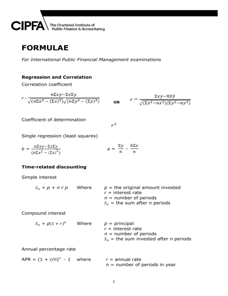
FORMULAE
For International Public Financial Management examinations
Regression and Correlation
Correlation coefficient
r=
Coefficient of determination
r=
OR
Single regression (least squares)
b=
ΣΣΣ
2
Σ2Σ a=
–
Time-related discounting
Simple interest
= p + n r p
Where
p = the original amount invested
r = interest rate
n = number of periods
= the sum after n periods
Where
p = principal
r = interest rate
n = number of periods
= the sum invested after n periods
Compound interest
= p1 Annual percentage rate
APR = (1 + r/n)n - 1
where
r = annual rate
n = number of periods in year
1
Daily percentage rate
K = 1 – 1
Where
K is the daily interest rate
R is the rate given
D is the number of days it relates to
Where
PV = present value
Discount factor
PV =
r = interest rate
n = number of periods
!the sum invested after n periods
Internal rate of return by interpolation
IRR = A+
"
"#
x (B-A) Where
A = lower discount rate
B = higher discount rate
C = NPV at lower discount rate
D = NPV at higher discount rate
Real rate of interest
()*+,+-.
$%&%'$ ! -/.*0,+-*(+-.
1
Equity cost of capital
Dividend valuation model:
!
1
Where
23
r=
shareholder’s cost of capital
d = annual dividend per share
MV = ex dividend share price
Dividend growth model:
=
1(4
23
+g
Where
r = the shareholders cost of capital
do = current dividend (net)
g = expected annual growth in
dividend payments (%)
MV = current ex div market price
2
Cost of debt capital and preference shares
i=
5
8( = current market price of debt capital
Where
67
K = the interest (dividend) received
i = the cost of debt (preference share)
capital
Capital asset pricing model
9 = 0 + β() -0 9
or :;
0 or 0
) or :)
β or B
Where
:; = 0 + (:) - 0 )B
or
=
=
=
=
the
the
the
the
expected return/cost of capital
risk free rate of return
return on the market portfolio
Beta factor of the individual security
Stock control and cash management
Economic Order Quantity
q=<
"#
Where
=
q = Economic Order Quantity
C = order cost
D = annual demand
H = stock holding cost per unit per annum
Reorder level model
Reorder level (ROL) = Lead time x Demand per time unit + safety stock
Miller-Orr model
B
z= <
>?@ A5
+L
Where
K = daily opportunity cost of cash
F = transaction cost
G = variance of net daily cash flows
Z = target balance
C ! 3E 2F
W=
AHI
H = upper limit
>
L = Lower limit
W = average balance
3
Baumol Model - Optimal cash injection
C=<
*
Where
C = cash injection
b = brokers’ fees
t = net cash flow over the period
i = opportunity cost of interest forgone
or cost of borrowing to provide funds
4