Journal of Hydrology 378 (2009) 161–167
Contents lists available at ScienceDirect
Journal of Hydrology
journal homepage: www.elsevier.com/locate/jhydrol
Estimating the snow water equivalent from snow depth measurements
in the Swiss Alps
T. Jonas *, C. Marty, J. Magnusson
WSL Institute for Snow and Avalanche Research SLF, Flüelastr. 11, 7260 Davos, Switzerland
a r t i c l e
i n f o
Article history:
Received 1 April 2009
Received in revised form 10 August 2009
Accepted 5 September 2009
This manuscript was handled by
K. Georgakakos, Editor-in-Chief
Keywords:
Snow hydrology
Mountain water resources
Seasonal snow
Spatiotemporal variability
Switzerland
s u m m a r y
The snow water equivalent (SWE) characterizes the hydrological significance of snow cover. However,
measuring SWE is time-consuming, thus alternative methods of determining SWE may be useful. SWE
can be calculated from snow depth if the bulk snow density is known. Thus, a reliable estimation method
of snow densities could (a) potentially save a lot of effort by, at least partly, sampling snow depth instead
of SWE, and would (b) allow snow hydrological evaluations, when only snow depth data are available. To
generate a useful parameterization of the bulk density a large dataset was analyzed covering snow densities and depths measured biweekly over five decades at 37 sites throughout the Swiss Alps. Four factors
were identified to affect the bulk snow density: season, snow depth, site altitude, and site location. These
factors constitute a convenient set of input variables for a snow density model developed in this study.
The accuracy of estimating SWE using our model is shown to be equivalent to the variability of repeated
SWE measurements at one site. The technique may therefore allow a more efficient but indirect sampling
of the SWE without necessarily affecting the data quality.
Ó 2009 Elsevier B.V. All rights reserved.
Introduction
Under a changing climate, mountain water resources become
increasingly important. In mountainous catchments snowmelt
typically constitutes a significant part of the total runoff (Barnett
et al., 2005; Hock et al., 2006). Therefore, keeping track of the spatial and temporal distribution of snow is vital for monitoring
mountain water resources and predicting subsequent runoff. For
hydrological applications, we need to characterize the snow cover
by its snow water equivalent (SWE).
Measuring SWE requires substantially more effort than it does
to sample snow depth. However, as will be shown later, SWE is
strongly correlated to the snow depth (HS). This correlation could
potentially be used to estimate SWE from HS. Thus, studies have
suggested enhancing sampling efficiency by substituting a significant part of the time-consuming SWE measurements by simple HS
measurements (Elder et al., 1998; Rovansek et al., 1993). However,
here we shall try to completely abandon SWE measurements and
assess that parameter from HS sampling alone.
The ratio SWE/HS at a single point is referred to as bulk snow
density (qb),
SWE ¼ HS qb
ð1Þ
Thus, estimating SWE from HS is the same task as estimating qb.
Sturm et al. (2009) recently came up with a qb model with respect
to snow depth and snow class (Sturm et al., 1995). Their study was
based on over 25,000 SWE–HS–qb records measured in several
countries over several decades. Here, we specifically address a regional parameterization of qb for seasonal snow in the Swiss Alps
that emphasizes the temporal evolution of qb.
Given the complex topography and frequent snow redistribution processes in alpine environments, SWE typically displays a
considerable spatial variability even within a given sample site
(Bray, 1973; Liston and Sturm, 2002). Hence, to establish a SWE value representative of such a site, several SWE measurements would
be necessary (Watson et al., 2006). However, with special regard to
catchment-scale water resource monitoring, such an effort seems
unrealistic and we shall regard the expenditure of one SWE measurement per site as a practical limit. Here, we hypothesize that
a few HS measurements converted to SWE using the proposed qb
model characterize a site as good as a single SWE measurement
but at less effort. This would allow putting the freed resources in
sampling at more sites. Moreover, the approach would also include
the possibility to convert historic HS data into SWE in the absence
of other information than sampling date and location.
Snow data
* Corresponding author. Tel.: +41 81 417 0259; fax: +41 81 417 0110.
E-mail addresses: jonas@slf.ch (T. Jonas), marty@slf.ch (C. Marty), magnusson@slf.ch (J. Magnusson).
0022-1694/$ - see front matter Ó 2009 Elsevier B.V. All rights reserved.
doi:10.1016/j.jhydrol.2009.09.021
The WSL Institute for Snow and Avalanche research SLF runs an
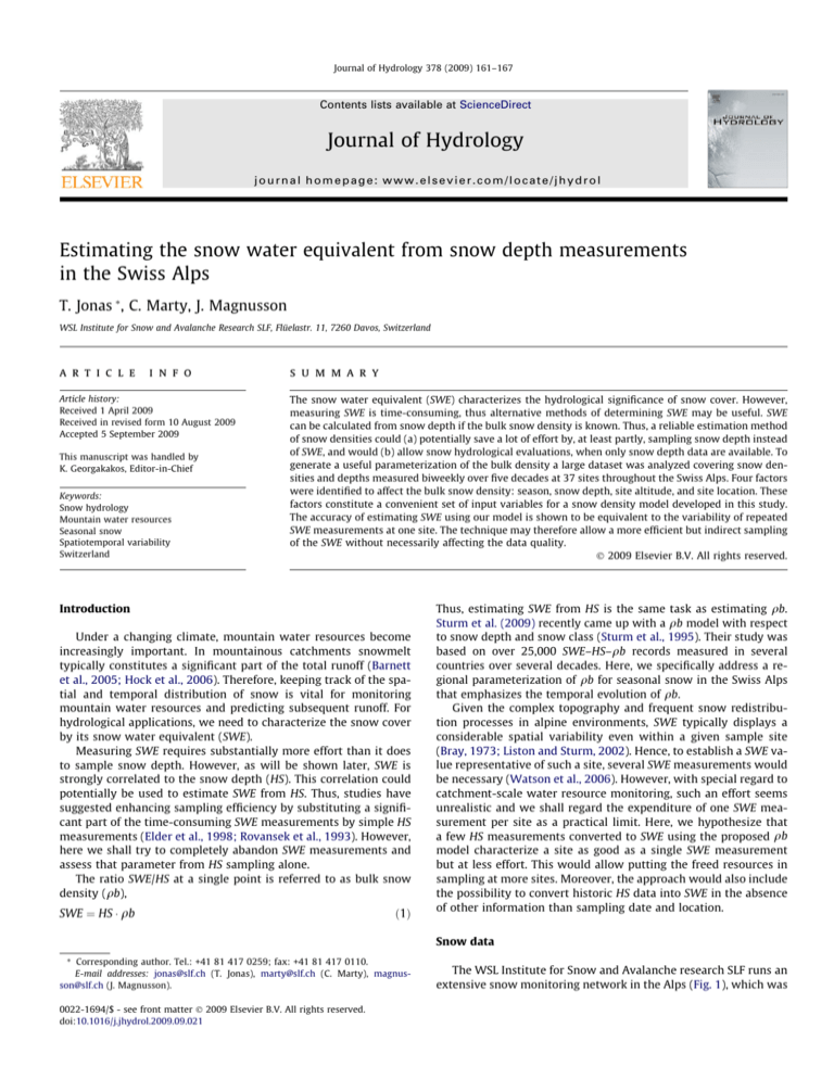
extensive snow monitoring network in the Alps (Fig. 1), which was
162
T. Jonas et al. / Journal of Hydrology 378 (2009) 161–167
erably from year to year and from site to site (data not shown).
Accumulation and melting of snow follows amongst other factors
the precipitation and temperature patterns (Elder et al., 1991; Laternser and Schneebeli, 2003).
Relationship between water equivalent, density, and depth of
snow
Fig. 1. Snow station sites and regions in Switzerland.
initiated about six decades ago by the Swiss Federal Institute of
Technology (ETH). SWE is sampled biweekly (i.e. twice a month)
by professional staff, all trained to the same standards. Snow cores
are taken using aluminum cylinders with a cross-sectional area of
70 cm2. On principle, a pit is dug to ensure that no snow is lost
when extracting the core from the snow cover (i.e. the core is taken
outside the pit and extracted laterally into the pit). Moreover, this
procedure ensures most accurate simultaneous HS measures on
the same spot. The measuring sites are typically flat and open. Note
that although qb is calculated from HS and SWE and thus not measured directly, HS/SWE will be referred to as the observed qb in the
following.
From our database we selected only records from sites that provided continuous long-term datasets of at least 20 years (on average 35 years) and followed the regular sampling scheme. This
selection procedure resulted in 11,147 SWE-HS-qb data records
from 48 winters (1960–2008) and 37 stations throughout the
Swiss Alps (Fig. 1). The sites cover an altitudinal range of 860–
2690 m asl. However, note that for historical reasons the majority
of the sites are located below 2000 m asl. Automatic plausibility
checks consisted of testing the data records to satisfy Eq. (1). Furthermore data with qb below 50 and above 600 kg/m3, respectively, were discarded.
The SLF distinguishes between seven snow-climate regions in
the Swiss Alps (Fig. 1). They reflect typical regional patterns in
snow cover climatology. As the region assignment constitutes a potential qb model input, all data have been attributed to their
respective region via site location.
The systematic snow samples resulted in typical distributions of
SWE, HS, and qb values: While the qb data are approximately normally distributed, SWE and HS data clearly exhibit a log-normal
distribution (Fig. 2). The evolution of the snow cover varies consid-
Snow depth, bulk density and water equivalent are related to
one another according to Eq. (1). The pair-wise correlations between these three snow cover properties are presented in Fig. 3.
As expected, SWE and HS display a strong correlation, which seems
approximately linear (Fig. 3a). However, on closer examination the
best-fit line is slightly curved upward. This statement is identical
to the finding that the mean qb increases with HS (Fig. 3b; Lundberg et al., 2006; Marchand and Killingtveit, 2004; Pomeroy and
Gray, 1995). qb was fitted to HS using a power curve (Fig. 3b),
qb ¼ 60:1 HS0:89 þ 237
ð2Þ
Multiplying this equation with HS results in a corresponding fit for
SWE to HS (Fig. 3a),
SWE ¼ ð60:1 HS0:89 þ 237Þ HS
ð3Þ
where in both Eqs. (2) and (3) SWE is in kg/m2, HS in m, and qb in
kg/m3.
The variance of the data shown is clearly non-uniform (i.e. heteroscedastic). In particular, a meaningful density model needs to
cope with the pronounced variability of qb at low snow depths.
A reason for this behavior is that a shallow snow cover can range
from low-density new snow in autumn to high-density slush in
spring. We may therefore expect a seasonal evolution of qb.
A direct plot of qb versus time shows that the bulk density gradually increases over the course of the winter season (Fig. 4a). This
effect has been reported by many previous studies (Anderton et al.,
2004; Elder et al., 1991; Mizukami and Perica, 2008; Rohrer et al.,
1994; Sturm and Holmgren, 1998) and corresponds to the increasing compaction of snow due initially to settling and later to snow
cover ripening. A relevant implication of the seasonal evolution
of qb is the distinct shape of the SWE-HS trajectories (Fig. 4b). Comparing these trajectories with the data shown in Fig. 3a, reveals
that accounting for the seasonal evolution of qb provides a promising tool to enhance SWE estimations from HS.
Besides time of the year and HS there are many other factors
that may potentially enhance the accuracy of qb estimations. However, to stay in line with the purpose of this paper we shall concentrate on factors that are accessible without substantial extra effort.
One of these easy-to-gather factors is the site location. The effect of
location was tested by considering region (Fig. 1) and altitude.
Fig. 2. Distribution of SWE, HS, and qb data sampled biweekly at 37 sites throughout the Swiss Alps over five decades (n = 11,147).
T. Jonas et al. / Journal of Hydrology 378 (2009) 161–167
163
Fig. 3. The relationship between SWE, qb, and HS. The best-fit lines are specified in Eqs. (2) and (3).
Fig. 4. The effect of season on bulk snow density. Panel b displays typical seasonal SWE–HS trajectories (exemplary data from station Weissfluhjoch at 2560 m asl.). Light to
dark gray colors denote months November–June.
Not surprisingly, there were considerable differences between
regions with regards to mean snow depths (not shown). These
findings can be linked to the precipitation and temperature patterns in Switzerland (Laternser and Schneebeli, 2003). However,
mean bulk densities differed only slightly between regions. Expect-
edly, regions #4, #5, and #7 displayed the lowest mean qb, as they
are dominated by a dry, inner-alpine climate.
The altitude has only a minor direct effect on the average qb
(Fig. 5a). This result may appear rather counter-intuitive, as higher snow depths at higher sites should entail increased mean qb.
164
T. Jonas et al. / Journal of Hydrology 378 (2009) 161–167
Fig. 5. The effect of altitude on bulk snow density. Distribution of qb data split up into altitudinal subsets, seasonal subsets, respectively. Box plots display the median value
±1 standard deviation, the whiskers denote median ±2 standard deviations. Data in panel b are staggered with respect to site altitude (left: P2000 m; center: P1400 m and
<2000 m; right: <1400 m).
Warmer temperatures at lower altitudes may, however, induce a
compensating effect (cf. Onuchin and Burenina, 1996). Nevertheless, altitude remains an interesting variable with respect to the
qb model. The interaction between the factors altitude and season
reveals an indirect effect on qb (Fig. 5b; see also Mizukami and
Perica, 2008). The data show that in early winter qb increases
with altitude, which is likely related to the fact that at this time
of the year only higher altitudes feature considerable snow
depths. However, in late winter the opposite is the case, and qb
decreases with altitude, because the melt-out progresses faster
at lower altitudes.
Further, sun exposure was tested for its direct or indirect effects
on qb. All the sites were manually classified as sun-exposed, normal, or shady. However, we did not find any considerable difference between these three classes with respect to qb.
Parameterization of the bulk snow density
The main purpose of the qb model is to facilitate SWE monitoring on the catchment scale. It should allow converting measured
HS values into SWE. However, to be an efficient technique the model should only require input data that can be recorded during a HS
survey with little additional effort. Clearly, for some applications
factors such as local insolation charts or previous meteorological
conditions are too laborious to handle or unavailable. Moreover,
the model needs to be applicable at other sites and to other times
than those covered by our dataset, i.e. year and site identifier are
not appropriate input factors either.
Thus far, four factors could be identified with a notable effect on
qb: (1) season, (2) HS, (3) site altitude, and (4) region. Gathering
these factors only requires recording location and date when sampling HS. Therefore, they are appropriate input factors for the qb
model.
Given the complex non-linear and interacting relationship between the four input factors and qb, we opted for a model combin-
ing the flexibility of look-up tables with the efficiency of data
fitting. In a first step the dataset was split up into three times 12
subsets (cf. Fig. 5b) according to three altitude range classes
(P2000 m, P1400 m and <2000 m, <1400 m) and 12 seasonal classes (months), respectively. Then, qb was fitted to HS data for each
data subset separately using linear regression. Non-linear regression did not enhance the fit; neither did fitting to log-transformed
HS data (cf. Fig. 2b). For simplicity, we retained the linear model
approach. The procedure resulted in two regression coefficients
per subset (Table 1). The table allows an estimation of preliminary
qb values from HS data
qbprel: ¼ a HSobs: þ b;
ð4Þ
where [b, a] are to be selected from Table 1 according to site altitude and recording date.
The preliminary qb model accounts for three out of four designated input factors, with region not yet included. Therefore, the full
dataset has been split up in seven subsets according to the regions
defined in Fig. 1. Per subset the model residuals qbprel.–qbobs. were
calculated and averaged yielding region-specific density offsets
(Table 2). These offset values may be used to enhance qb estimations in Switzerland according to
qbmod: ¼ a HSobs: þ b þ offsetreg: ;
ð5Þ
where offsetreg. is to be selected from Table 2 according to region.
Finally, SWE can be deduced as
SWEmod: ¼ HSobs: qbmod:
ð6Þ
The type of model may appear simplistic. However, the combination of look-up tables with regression analysis allows reflecting
the complex and non-linear interactions between the four terms
with relevant effects on qb, while at the same time the application
remains user friendly.
165
T. Jonas et al. / Journal of Hydrology 378 (2009) 161–167
Table 1
Look-up table for regression coefficients [b, a]. The bulk snow density can be calculated from snow depth according to Eq. (4). (n, R) denote the number of data records used for the
regressions and the correlation coefficients in %, respectively.
October
November
December
January
February
March
April
May
June
July
a
Altitudes (asl.) P2000 m [b, a]; (n, R)
Altitudes (asl.) P1400 m and <2000 m [b, a]; (n, R)
Altitudes (asl.) <1400 m [b, a]; (n, R)
na.a
[206, 47]; (116, 27)
[203, 52]; (237, 45)
[206, 52]; (234, 58)
[217, 46]; (235, 53)
[272, 26]; (247, 38)
[331, 9]; (214, 13)
[378, 21]; (124, 22)
[452, 8]; (81, 11)
[470, 15]; (22, 20)
na.
[183, 35];
[190, 47];
[208, 47];
[218, 52];
[281, 31];
[354, 15];
[409, 29];
na.
na.
na.
[149, 37]; (141, 14)
[201, 26]; (625, 13)
[235, 31]; (866, 18)
[279, 9]; (916, 6)
[333, 3]; (826, 2)
[347, 25]; (451, 17)
[413, 19]; (88, 11)
na.
na.
(198, 16)
(864, 31)
(1145, 35)
(1198, 48)
(1218, 29)
(828, 14)
(273, 26)
Too little data available to establish a regression model.
Table 2
Look-up table for region-specific offsets, cf. Eq. (5). n denotes the number of data
records available per region.
Region
3
Offset (kg/m )
n
1
2
3
4
5
6
7
+7.6
893
+11.7
2989
+11.8
1171
1.1
1535
0.3
2330
+12.1
535
14.7
1694
Model test
The model was evaluated in several ways: using in-sample
tests, analyzing the model’s transferability to independent data,
and by testing the effect of model simplifications. As a first test
of the model performance, qbmod. and SWEmod. were calculated
from the observed HS data and compared to qbobs. and SWEobs.,
respectively (Fig. 6). While the bulk of the estimated qb data (±1
standard deviation) matches the observed data within a range of
±45 kg/m3, the scatter of the residuals is considerable (Fig. 6a).
However, this finding is not astonishing, as the model was not de-
signed to account for previous meteorological conditions that governs the evolution of the snowpack sampled (Meloysund et al.,
2007; Onuchin and Burenina, 1996; Sturm and Holmgren, 1998).
Especially in lower regions, the meteorological history is decisive
(Rohrer et al., 1994). Accordingly, specific error bounds for a data
subset from lower sites display a greater model uncertainty than
respective results for sites at higher altitudes. As for the SWE, estimated values compare well with observed data (Fig. 6b). The bulk
of the estimates (±1 standard deviation) are on average within 16%
of the observed value, with a tendency for better results at high
SWE, worse results at low SWE respectively. The model performance with respect to SWE yields much better results than the
respective comparison for qb, which corresponds to the observation that most of the variability in SWE is explained by the variability of HS (Fig. 3a; Pomeroy and Gray, 1995).
To gain more insight into the model performance, we identified
those 10% of the qbmod. data with the highest bias relative to qbobs.,
termed as qbw10% in the following. It was then tested whether data
from specific months, altitudes, or snow depths were significantly
Fig. 6. Observed versus modeled bulk snow density and snow water equivalent, respectively. The solid blue lines indicate gliding prediction bounds corresponding to median,
±1 standard deviation (inner bounds), and ±2 standard deviations (outer bounds), respectively. (For interpretation of the references to colours in this figure legend, the reader
is referred to the web version of this paper).
166
T. Jonas et al. / Journal of Hydrology 378 (2009) 161–167
splitting (V2). Therefore, random 10% of the data were excluded
from the data pool for model calibration and subsequently used
as independent validation data. This step was repeated further nine
times, where as each dataset could only once be drawn for the
cross-validation. And third, the model was tested against 2188
datasets (V3) from snow stations that were excluded from the final
model calibration when their records did not meet the required
length of at least 20 years (cf. Snow data section). Note that a random draw procedure was applied to ensure the validation dataset
to feature the same snow depth distribution as shown in Fig. 2.
Additionally, the effect of simplifications of the final model on its
performance was tested (Table 3). Model simplifications A1–A5
were realized by neglecting the effects of season, site altitude,
snow depth, and site location on qbmod. separately or combinedly.
The model’s RMSE using the calibration data for validation (Table
3, V1) is used as the benchmark performance. The cross-validation
(V2) displays a practically identical performance, while the validation with alternative data (V3) results in a minor reduction of the
model performance. The model seems thus quite robust with respect to transferability to independent data. Remarkably, also the
alternative model A1 achieves a RMSE similar to the benchmark
performance. Obviously the effects of site altitude and location (in
Switzerland) are minor compared to the effects of season and snow
depth on qb. This finding suggests that the model presented in this
study may also be applicable to snow depth data from areas outside
the Swiss Alps, provided similar climatologic conditions. Even an
extrapolation to climate predicted for the near future may be
appropriate, since expected snow cover changes in the Alps seem
to resemble snow regimes existing today but at lower altitudes
(Bavay et al., 2009; Magnusson et al., 2009). The validation of alternative models A2–A4 reveals that neglecting either the effect of
snow depth or the effect of season on qb significantly increases
the model bias. Of these two effects the seasonal variation in qb
seems clearly more important for incorporation in the model. The
same conclusion can also be drawn when comparing the magnitude
of both effects in the respective univariate plots (Figs. 3b and 4a).
Table 3
Model test: RMSE of SWEmod. – SWEobs. using different validation datasets (V1–V3) and
alternative models (A1–A5). Validation datasets for model configurations V1–V3 are
described in the section Model test. Alternative models A1–A5 were tested against the
full dataset, where the table specifies (), which of the four available effects were
accounted for.
a
b
Model
Month
Altitude
HS
Region
RMSE
V1
V2
V3
A1
A2
A3
A4a
A5b
50.9
51.3
53.2
53.3
58.1
73.0
72.3
88.7
qbmod. according to Eq. (2).
Model uses a constant qbmod. = median (qbobs.).
overrepresented in qbw10%. With respect to season, the analysis revealed that only qb predictions for November were overrepresented in the subsample with the highest bias (20% of all
November data were contained in qbw10%). November had the
highest variability in observed qb with snow types ranging from
light new snow to melting ephemeral snow. Similarly, the lowest
altitudes displayed higher bias of qbmod. (22% of all data sampled
below 1000 m asl. were contained in qbw10%). While at higher altitudes the snow season typically displays a clearly defined accumulation period followed by the ablation period, at lower altitudes
melting may occur episodically throughout the entire snow season,
which causes greater variability in observed qb. Finally, shallow
snowpacks were overrepresented in the subsample with the highest bias of qbmod. (23% of all data with HS < 0.25 m, were contained
in qbw10%). This effect could be attributed to the lowest values of
qbobs., which invariably occurred at low snow depths, where these
extreme values seem difficult to capture by a stochastic approach.
Summarizing and not astonishing, the model displays notable difficulties to predict qbmod. for low-altitude, early-season, and shallow snowpacks. These circumstances favor the occurrence of
ephemeral snow, the density of which is hard to predict without
accounting for previous meteorological conditions.
To test the transferability of the model to independent data,
qbmod. and SWEmod. from observed HS data were compared to qbobs.
and SWEobs. using three configurations of model calibration data
versus model validation data (Table 3): first, all data used to calibrate the final model above were also used for validation (V1). Second, the model was cross-validated using a tenfold 90%/10% data
Utility of the model
It was initially hypothesized that a few HS measurements converted to SWE using the qb model characterize a site as good as a
single SWE measurement but at less effort. To test the hypothesis,
the model residuals are compared to the variability of repeated
SWE measurements at one site. There is surprisingly little data
published on the within-site variability of both, SWE and qb. More-
Table 4
Within-site variability of bulk snow density and snow water equivalent according to literature and field experiments. A description of the studies (1)–(4) can be found in the
papers referenced below. The Swiss experiments were conducted nearby Davos on flat and open field sites between 1560 and 2200 m asl. using the same measurement
techniques as described in the section Snow data.
(1)
(2)
(3)
(4)
(5)
(6)
(7)
Citation
(1)
(2)
(3)
(4)
(5)
(5)
(5)
Country
Season
Approx. HS
Sampling spacing
Sampling design
Number of samples
HS compensation (6)
Variability qb (7)
Variability SWE (7)
USA
Mid winter
70 cm
10 m
100 m lines
1240
Yes
23%
23%
Canada
Diff. times
55 cm
1m
8 8 m grid
108
Yes
21%
21%
Canada
February
55 cm
Random
50 m radius
322
No
11–20%
23–27%
Canada
Pre-melt
—
5m
100 100 m grid
437
No
—
36–80%
Switzerland
Early winter
46 cm
5/10 m
25 25 m grid
18
No
8%
18%
Switzerland
Mid winter
152 cm
5/10 m
25 25 m grid
18
No
7%
13%
Switzerland
Late winter
51 cm
5m
25 25 m grid
36
No
15%
30%
Sturm and Liston, (2003).
Bray, (1973).
Kershaw and McCulloch, 2007).
Janowicz et al., (2003).
Own experiment.
Data was corrected with reference to site-averaged HSmean, i.e.: SWEcorr. = SWEi – (HSi–HSmean)qbmean; qbcorr. = SWEcorr./HSmean.
One standard deviation/mean.
T. Jonas et al. / Journal of Hydrology 378 (2009) 161–167
over, it is arguable whether respective results from different studies can be compared because of different length scales, different
snow regimes, and sampling techniques with different accuracies
involved. Nevertheless, Table 4 shall give a rough overview on
the within-site variability of SWE and qb.
The data compilation in Table 4, suggests that 10–20% is a typical range for the within-site variability of repeated qb measurements. Superposed variations in HS seem to augment the withinsite variability of SWE where a typical range may be conservatively
given as 15–25%. Comparing this number with the variance of the
model residuals (16%, Model test section), we may accept the initial hypothesis suggesting that the qb model in combination with
few HS measurements characterizes a site as well as a single SWE
measurement.
Note that the model may not be suitable to convert time series
of HS into SWE at daily resolution or higher. Transient phenomena
such as the settling of recently fallen fresh snow cannot be comprehended by the model. Converted time series may therefore feature an incorrect fine structure in the temporal course of SWE.
Conclusions
This study attempts to enhance estimations of the snow water
equivalent from snow depth observations on the condition that
no additional measurements shall be required. Given Eq. (1), this
task corresponds to finding a feasible parameterization of the bulk
snow density. We therefore investigated how the bulk snow density is affected by snow depth and other factors that could be derived from recording date and location. The analysis is based on
11,147 records of snow densities and depths measured over five
decades at 37 sites throughout the Swiss Alps.
Four factors were identified to feature a relevant effect on bulk
snow density, which are (ordered by relevance): season, snow
depth, site altitude, and snow-climate region. These factors were
consequently used as input for a new bulk snow density model primarily applicable to seasonal snow in the Swiss Alps. However, the
minor importance of regional effects suggests that the model may
also be applicable in other regions with similar snow climatologic
conditions. The model combines look-up tables with regression
analysis and is very easy to use.
Applying the model to different datasets of combined snow
depth and water equivalent measurements enabled comparing
estimated snow densities with corresponding verification data.
The model uncertainty was found to be of the same order of magnitude as the variability of repeated measurements at one site. We
hence conclude that modeled bulk densities and snow water
equivalents can represent a given site as well as respective single-point measurements. Depending on the application, this approach may consequently allow substituting time-consuming
snow water equivalent measurements by a few snow depth
samples.
Acknowledgements
We wish to thank all known and unknown colleagues that were
involved in collecting the snow data over five decades, without
whom this study would not have been possible. Data from three
167
out of 37 snow stations were provided by Mario Rohrer. We also
thank Manfred Stähli, Ethan M. Greene, Martin Schneebeli, Noah
Molotch, and Keith Musselman for their helpful comments on this
manuscript.
References
Anderton, S.P., White, S.M., Alvera, B., 2004. Evaluation of spatial variability in snow
water equivalent for a high mountain catchment. Hydrological Processes 18 (3),
435–453.
Barnett, T.P., Adam, J.C., Lettenmaier, D.P., 2005. Potential impacts of a warming
climate on water availability in snow-dominated regions. Nature 438 (7066),
303–309.
Bavay, M., Lehning, M., Jonas, T., Lowe, H., 2009. Simulations of future snow cover
and discharge in Alpine headwater catchments. Hydrological Processes 23 (1),
95–108.
Bray, D.I., 1973. A report on the variability of snow water equivalent measurements
at a site. In: In: Proceedings of the 30th Eastern Snow Conference, pp. 20–31.
Elder, K., Dozier, J., Michaelsen, J., 1991. Snow accumulation and distribution in an
Alpine watershed. Water Resources Research 27 (7), 1541–1552.
Elder, K., Rosenthal, W., Davis, R.E., 1998. Estimating the spatial distribution of snow
water equivalence in a montane watershed. Hydrological Processes 12 (10–11),
1793–1808.
Hock, R., Rees, G., Williams, M.W., Ramirez, E., 2006. Preface – contribution from
glaciers and snow cover to runoff from mountains in different climates.
Hydrological Processes 20 (10), 2089–2090 (special issue).
Janowicz, J.R., Gray, D.M., Pomeroy, J.W., 2003. Spatial variability of fall soil
moisture and spring snow water equivalent within a mountainous Sub-Arctic
watershed. In: Proceedings of the 60th Eastern Snow Conference, pp. 127–139.
Kershaw, G.P., McCulloch, J., 2007. Midwinter snowpack variation across the Arctic
treeline, Churchill, Manitoba, Canada. Arctic Antarctic and Alpine Research 39
(1), 9–15.
Laternser, M., Schneebeli, M., 2003. Long-term snow climate trends of the Swiss
Alps (1931–99). International Journal of Climatology 23, 733–750.
Liston, G.E., Sturm, M., 2002. Winter precipitation patterns in arctic Alaska
determined from a blowing-snow model and snow-depth observations.
Journal of Hydrometeorology 3 (6), 646–659.
Lundberg, A., Richardson–Naslund, C., Andersson, C., 2006. Snow density variations:
consequences for ground-penetrating radar. Hydrological Processes 20 (7),
1483–1495.
Magnusson, J., Jonas, T., Lopez-Moreno, J.I., Lehning, M., 2009. Snow cover response
to climate change in a high alpine and half glaciated basin in Switzerland.
Hydrology Research, accepted for publication.
Marchand, W.D., Killingtveit, A., 2004. Statistical properties of spatial snowcover in
mountainous catchments in Norway. Nordic Hydrology 35 (2), 101–117.
Meloysund, V., Leira, B., Hoiseth, K.V., Liso, K.R., 2007. Predicting snow density using
meteorological data. Meteorological Applications 14 (4), 413–423.
Mizukami, N., Perica, S., 2008. Spatiotemporal characteristics of snowpack density
in the mountainous regions of the Western United States. Journal of
Hydrometeorology 9 (6), 1416–1426.
Onuchin, A.A., Burenina, T.A., 1996. Climatic and geographic patterns in snow
density dynamics, Northern Eurasia. Arctic and Alpine Research 28 (1), 99–103.
Pomeroy, J.W., Gray, D.M., 1995. Snow Accumulation, Relocation and Management.
National Hydrology Research Institute Science Report No. 7, p. 144.
Rohrer, M., Braun, L.N., Lang, H., 1994. Long-term records of snow cover water
equivalent in the Swiss Alps: 1. Analysis.. Nordic Hydrology 25, 53–64.
Rovansek, R.J., Kane, D.L., Hinzman, L.D., 1993. Improving estimates of snowpack
water equivalent using double sampling. In: In: Proceedings of the 61st
Western Snow Conference, pp. 157–163.
Sturm, M., Holmgren, J., 1998. Differences in compaction behaviour of three climate
classes of snow. Annals of Glaciology 26, 125–130.
Sturm, M., Holmgren, J., Liston, G.E., 1995. A seasonal snow cover classification
system for local to global applications. Journal of Climate 8 (5), 1261–1283.
Sturm, M., Liston, G.E., 2003. The snow cover on lakes of the Arctic Coastal Plain of
Alaska, USA. Journal of Glaciology 49 (166), 370–380.
Sturm, M. et al., submitted for publication. Estimating local to global snow water
resources using snow depth data and snow climate classes. Journal of
Hydrometeorology.
Watson, F.G.R., Anderson, T.N., Newman, W.B., Alexander, S.E., Garrott, R.A., 2006.
Optimal sampling schemes for estimating mean snow water equivalents in
stratified heterogeneous landscapes. Journal of Hydrology 328 (3–4), 432–452.