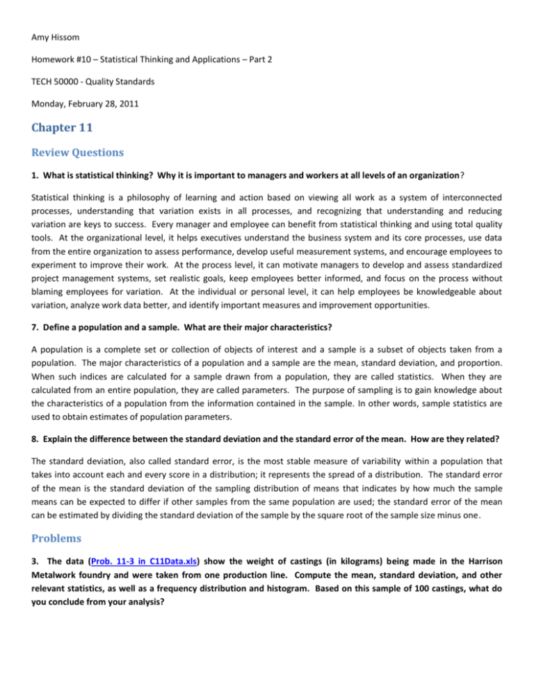
Amy Hissom
Homework #10 – Statistical Thinking and Applications – Part 2
TECH 50000 - Quality Standards
Monday, February 28, 2011
Chapter 11
Review Questions
1. What is statistical thinking? Why it is important to managers and workers at all levels of an organization?
Statistical thinking is a philosophy of learning and action based on viewing all work as a system of interconnected
processes, understanding that variation exists in all processes, and recognizing that understanding and reducing
variation are keys to success. Every manager and employee can benefit from statistical thinking and using total quality
tools. At the organizational level, it helps executives understand the business system and its core processes, use data
from the entire organization to assess performance, develop useful measurement systems, and encourage employees to
experiment to improve their work. At the process level, it can motivate managers to develop and assess standardized
project management systems, set realistic goals, keep employees better informed, and focus on the process without
blaming employees for variation. At the individual or personal level, it can help employees be knowledgeable about
variation, analyze work data better, and identify important measures and improvement opportunities.
7. Define a population and a sample. What are their major characteristics?
A population is a complete set or collection of objects of interest and a sample is a subset of objects taken from a
population. The major characteristics of a population and a sample are the mean, standard deviation, and proportion.
When such indices are calculated for a sample drawn from a population, they are called statistics. When they are
calculated from an entire population, they are called parameters. The purpose of sampling is to gain knowledge about
the characteristics of a population from the information contained in the sample. In other words, sample statistics are
used to obtain estimates of population parameters.
8. Explain the difference between the standard deviation and the standard error of the mean. How are they related?
The standard deviation, also called standard error, is the most stable measure of variability within a population that
takes into account each and every score in a distribution; it represents the spread of a distribution. The standard error
of the mean is the standard deviation of the sampling distribution of means that indicates by how much the sample
means can be expected to differ if other samples from the same population are used; the standard error of the mean
can be estimated by dividing the standard deviation of the sample by the square root of the sample size minus one.
Problems
3. The data (Prob. 11-3 in C11Data.xls) show the weight of castings (in kilograms) being made in the Harrison
Metalwork foundry and were taken from one production line. Compute the mean, standard deviation, and other
relevant statistics, as well as a frequency distribution and histogram. Based on this sample of 100 castings, what do
you conclude from your analysis?
Descriptive Statistics
Harrison Metalwork Foundry Production Line 1
Frequency Distribution
Weight of Castings (kilograms) Based on a Sample of 100
23
25
23
6
3
39.9
39.6
39.3
39
38.7
38.4
1
38.1
1
Frequenci…
10
8
37.8
30
25
20
15
10
5
0
37.5
38.6700
0.0456
38.7000
38.4000
0.4556
0.2076
0.3747
-0.1715
2.6000
37.3000
39.9000
3867.0000
100.0000
0.0904
Frequency
Mean
Standard Error
Median
Mode
Standard Deviation
Sample Variance
Kurtosis
Skewness
Range
Minimum
Maximum
Sum
Count
Confidence Level (95.0%)
Boundaries
The descriptive statistics and histogram that I computed from the raw data in Prob. 11-3 in C11Data.xls using Excel’s
analysis tools is shown below. Based on the sample of 100 castings obtained from Harrison Metalwork Foundry’s
production line, I would say that although there is a minor skewing to the right, the distribution of the data seems to be
fairly normal.
7. Outback Beer bottles have been found to have a standard deviation of 5 ml. If 95 percent of the bottles contain
more than 230 ml, what is the average filling volume of the bottles?
If, σ = 5 ml. x = 230, and P (z>x) =0.95
Since, 0.5000-0.9500=0.45, then based on the z-chart, z = -1.6455.
So, if 1.6455 x 5 = 8.2275
And
Then
µ = 238.2275
Therefore,
µ = 238.228 ml. is the average filling volume of the bottles.
This is where I am a little confused on rounding the number. Is µ actually 238.228 or is it 238.223?
11. In a filling line at A & C Foods, Ltd., the mean fill volume for rice bubbles is 475 grams and the standard deviation
is 10 grams. What percentage of containers will have less than 450 grams More than 485 grams (assuming no
overflow)?
If, µ = 475 grams and σ = 10 grams, then to show the percentage of containers having less than 450 grams:
P(x<450) = 0.5000 – P (450< x <475)
So, using the z-chart: P (z<450) = 0.5000- 0.4798=0.0202
Therefore, 2.02% of the containers will have less than 450 grams.
If, µ = 475 grams and σ = 10 grams, then to show the percentage of containers having more than 485 grams:
P(x>485) = 0.5000 – P (475< x <485)
So, using the z-chart: P (z>485) = 0.5000- 0.3413= 0.1587
Therefore, 15.87% of the containers will have more than 485 grams.
12. The frequency table that follows shows the weight of castings (in kilograms) being made at the Harrison
Metalwork foundry after process changes took place (see Prob. 11-3, in C11Data.xls, for “raw” data).
Frequency Table
Upper Cell
Frequencies
Boundaries
37.5
1
37.8
3
38.1
8
38.4
23
38.7
25
39.0
23
39.3
10
39.6
6
39.9
1
Cell
Cell 1
Cell 2
Cell 3
Cell 4
Cell 5
Cell 6
Cell 7
Cell 8
Cell 9
Cell
Adjusted Cell Midpoints
37.35
37.65
37.95
38.25
38.55
38.85
39.15
39.45
39.75
Cell 1
Cell 2
Cell 3
Cell 4
Cell 5
Cell 6
Cell 7
Cell 8
Cell 9
Frequencies
1
3
8
23
25
23
10
6
1
Cumulative %
1.00%
4.00%
12.00%
35.00%
60.00%
83.00%
93.00%
99.00%
100.00%
fx
37.35
112.95
303.60
879.75
963.75
893.55
391.50
236.70
39.75
fx^2
1395.02
4252.57
11521.62
33650.44
37152.56
34714.42
15327.23
9337.82
1580.06
3858.90
148931.73
a) Based on this sample of 100 castings, find the mean and standard deviation of the sample. (Note: If only
the given data are used, it will be necessary to research formulae for calculating the mean and standard
deviations using grouped data from a statistics text.)
̅
∑
√∑
∑
√
√
Source: www.drweedman.com/Mean.doc
Based on the adjusted midpoints the mean is 38.589 and the standard deviation is 0.4566 opposed to the descriptive
statistics on the Excel spreadsheet for problems #3 that shows the mean as 38.670 and the standard deviation as
0.4556.
Again I am confused on rounding. Is the answer 0.4566 or is it 0.457?
b) Use an Excel spreadsheet, if not already done for problem 11-3, to plot the histogram for the data.
Please see problem #3 above and attached Excel file.
c) Plot the data on normal probability paper to determine whether the distribution of the data is
approximately normal. (Note: The Regression tool in Excel has a normal probability plot that may be
used here.)
Y
Looking at the following plot chart, I would say the distribution of the data is approximately normal.
40.5
40.0
39.5
39.0
38.5
38.0
37.5
37.0
0.0000
Normal Probability Plot
20.0000
40.0000
60.0000
80.0000
100.0000
Sample Percentile
15. Determine the approximate sample size to estimate the proportion of sorting errors at a post office at a 99
percent confidence level. Historically, the sorting error rate is 0.0125, and you wish to have an allowable statistical
error of 0.01. (Note: Problems 15-19 address sample size determination and refer to theory covered in the Bonus
Material for this chapter as contained on the student CD-ROM.)
CI = 99%
z /2 = 2.58 (Since the value of “Z” based on the z-chart should be 2.58 for 99% confidence)(0.995)
p = 0.0125
1-p = 1 – 0.0125 = 0.9875
E = 0.01
So,
n = (z a/2)2 p (1-p) / E2
n = (2.58)2 (0.0125) (0.9875) / (0.01)2
n = 821.649375
n = 821.65
n = 822 as the approximate sample size.