Math 115
N. Psomas
Chapter 4 (Sections 4.3 - 4.4) Homework Solutions
Section 4.3
4.53 Discrete or continuous. In each of the following situations decide if the random variable is
discrete or continuous and give a reason for your answer.
(a) Your Web page has five different links and a user can click on one of the links or can
leave the page. You record the length of time that a user spends on the Web page before
clicking one of the links or leaving the page.
(b) The number of hits on your Web page.
(c) The yearly income of a visitor to your Web page.
Solution
(a) Continuous
(b) Discrete
(c) Book says discrete because income is measured to the nearest 100th of a dollar - nearest cent. For
most practical purposes though, it can be safely considered continuous.
4.54 Texas hold’em. The game of Texas hold’em starts with each player receiving two cards.
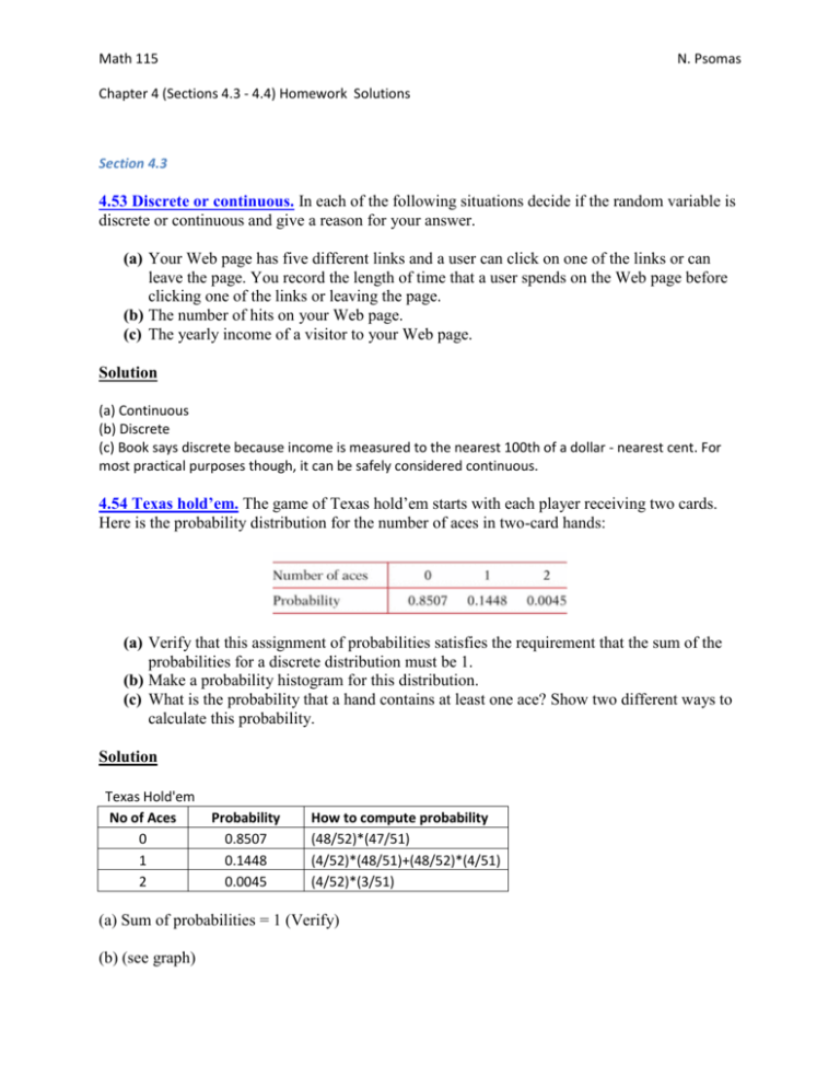
Here is the probability distribution for the number of aces in two-card hands:
(a) Verify that this assignment of probabilities satisfies the requirement that the sum of the
probabilities for a discrete distribution must be 1.
(b) Make a probability histogram for this distribution.
(c) What is the probability that a hand contains at least one ace? Show two different ways to
calculate this probability.
Solution
Texas Hold'em
No of Aces
0
1
2
Probability
0.8507
0.1448
0.0045
How to compute probability
(48/52)*(47/51)
(4/52)*(48/51)+(48/52)*(4/51)
(4/52)*(3/51)
(a) Sum of probabilities = 1 (Verify)
(b) (see graph)
(c) P(At least one Ace) = P(1 or 2 aces) = P(1) + P(2) = 0.1448 + 0.0045 = 0.1493
OR ... P(At least one Ace) = 1 - P(no aces) = 1 - 0.8507 = 0.1493
4.55 Spell-checking software. Spell-checking software catches “nonword errors,” which result
in a string of letters that is not a word, as when “the” is typed as “teh.” When undergraduates are
asked to write a 250-word essay (without spell-checking), the number X of nonword errors has
the following distribution:
(a) Sketch the probability distribution for this random variable.
(b) Write the event “at least one non-word error” in terms of X.
What is the probability of this event?
(c) Describe the event X ≤ 2 in words. What is its probability?
What is the probability that X < 2?
Solution
(a) See graph
(b) X > 0, or X ≥ 1
P(X > 0) = P(X ≥ 1) = P{1, 2, 3, 4} = 1 - P{0} = 1 - 0.1 = 0.9
(c) "At most 2 non-word errors"
P("At most 2 non-word errors") = P(X ≤ 2) = P{0, 1, 2} = 0.1 + 0.3 + 0.3 = 0.7
P( X < 2) = P{0, 1} = 0.1 + 0.3 = 0.4
4.56 Length of human pregnancies. The length of human pregnancies from conception to birth
varies according to a distribution that is approximately Normal with mean 266 days and standard
deviation 16 days. Call the length of a randomly chosen pregnancy Y.
(a) Make a sketch of the density curve for this random variable.
(b) What is P(Y ≤ 280)?
Solution
(a) See graph
(b) P( Y ≤ 280 ) = P(Z ≤ (280 - 266)/16 ) = P(Z ≤ .875)
= (.8078 + .8106)/2 = 0.8092
Note: Here because the z-value .875 happens to fall exactly in the middle of .87 and .88, the two
z-values listed in table A, averaging the probabilities listed in table A for z=.87 & z = .88 give a
more accurate value for P(Z ≤ .875).
Alternatively, use TI-83/84's normalcdf(a, b, µ, σ) function to compute P( Y ≤ 280 ).
normalcdf(0, 280, 266, 16) = 0.809213
4.57 Tossing two dice. Some games of chance rely on tossing two dice. Each die has six faces,
marked with 1, 2,…, 6 spots called pips. The dice used in casinos are carefully balanced so that
each face is equally likely to come up. When two dice are tossed, each of the 36 possible pairs of
faces is equally likely to come up. The outcome of interest to a gambler is the sum of the pips on
the two up-faces. Call this random variable X.
(a) Write down all 36 possible pairs of faces.
(b) If all pairs have the same probability, what must be the probability of each pair?
(c) Write the value of X next to each pair of faces and use this information with the result of
(b) to give the probability distribution of X. Draw a probability histogram to display the
distribution.
(d) One bet available in craps wins if a 7 or an 11 comes up on the next roll of two dice.
What is the probability of rolling a 7 or an 11 on the next roll?
(e) Several bets in craps lose if a 7 is rolled. If any outcome other than 7 occurs, these bets
either win or continue to the next roll. What is the probability that anything other than a 7
is rolled?
Solution
(a)
1
2
3
4
5
6
1
(1,1)
(1,2)
(1,3)
(1,4)
(1,5)
(1,6)
2
(2,1)
(2,2)
(2,3)
(2,4)
(2,5)
(2,6)
3
(3,1)
(3,2)
(3,3)
(3,4)
(3,5)
(3,6)
4
(4,1)
(4,2)
(4,3)
(4,4)
(4,5)
(4,6)
5
(5,1)
(5,2)
(5,3)
(5,4)
(5,5)
(5,6)
6
(6,1)
(6,2)
(6,3)
(6,4)
(6,5)
(6,6)
(b) 1/36
(c)
(d) P(7 or 11) = P(7) + P(11) = 0.1666667 + 0.0555556 = 0.22222
Note: Probability values shown on the histogram are rounded. If you use them to answer question (d)
the result will be slightly off. In this case 0.223.
(e) P(not a 7) = 1 - P(7) = 1 - 6/36 = 30/36 = .83333
Section 4.4
4.74 Mean of the distribution for the number of aces. In Exercise 4.54 you examined the
probability distribution for the number of aces when you are dealt two cards in the game of
Texas hold’em. Let X represent the number of aces in a randomly selected deal of two cards in
this game. Here is the probability distribution for the random variable X:
Find μX, the mean of the probability distribution of X.
Solution
μX = (0)(0.8507) + (1)(0.1448) + (2)(0.0045) = 0.1538
Note: This is the average number of aces a player is dealt in the long run.
4.75 Mean of the grade distribution. Example 4.22 gives the distribution of grades (A = 4, B =
3, and so on) in English 210 at North Carolina State University as
Find the average (that is, the mean) grade in this course.
Solution
μX = (0)(0.05) + (1)(0.04) + (2)(0.20) + (3)(0.40) + (4)(0.31) = 2.88
4.77 Standard deviation of the number of aces. Refer to Exercise 4.74. Find the standard
deviation of the number of aces.
No of Aces X
0
1
2
P(X)
0.8507
0.1448
0.0045
X*P(X)
0
0.1448
0.009
(X-µ)
P(X)*(X-µ)2
-0.1538 0.020122832
0.8462 0.103684683
1.8462 0.015338045
µ=
0.1538
σ2 = 0.13914556
σ = 0.373022198
Using TI-83/84
Enter the values of X in L1 & the probability for each value in L2
Press STAT > select CALC > Select 1: 1-Var Stats > Press Enter > Type L1,L2
Press Enter
4.78 Standard deviation of the grades. Refer to Exercise 4.75. Find the standard deviation of
the grade distribution.
Work as in Exercise 4.77
4.80 Find the mean of the sum. Figure 4.12 (page 259) displays the density curve of the sum Y
= X1 + X2 of two independent random numbers, each uniformly distributed between 0 and 1.
(a) The mean of a continuous random variable is the balance point of its density curve. Use
this fact to find the mean of Y from Figure 4.12.
(b) Use the same fact to find the means of X1 and X2. (They have the density curve pictured
in Figure 4.9, (page 254.) Verify that the mean of Y is the sum of the mean of X1 and the
mean of X2.
Figure 4.9
Figure 4.12
(a) By inspection (looking at Figure 4.12), the balance point is @ 1.
Therefore µY = X1 + X2 = 1.
(b) Similarly, the mean for X1 & X2 (µX1 & µX2 ) is 0.5
µY = X1 + X2 = µX1 + µX2
4.83 Means and variances of sums. The rules for means and variances allow you to find the
mean and variance of a sum of random variables without first finding the distribution of the sum,
which is usually much harder to do.
(a) A single toss of a balanced coin has either 0 or 1 head, each with probability 1/2. What
are the mean and standard deviation of the number of heads?
(b) Toss a coin four times. Use the rules for means and variances to find the mean and
standard deviation of the total number of heads.
(c) Example 4.23 (page 251) finds the distribution of the number of heads in four tosses.
Find the mean and standard deviation from this distribution. Your results in parts (b) and
(c) should agree.
Solution
(a) Here think of X as the variable that equals the # of heads you get when you toss a coin once.
X = 0 if tails shows up and X = 1 if heads shows up. With probabilities: P(0) = 1/2 & P(1) = 1/2
In summary:
X
P(X)
0
.5
1
.5
µX = .5 & σX = .5 (Use your calculator & work like in exercise 4.77)
(b) Here think of Y as the sum of four variables each having the same distribution as the variable
X in part (a). i.e. Y = X1 + X2 + X3 + X4
According to the rules for means and variances:
µy = µx1 + µx2 + µx3 + µx4
= 4*(.5) = 2
Var(Y) = Var(X1) + Var(X2) + Var(X3) + Var(X4) = 4* (.25) = 1 ; Note: Var(X) = (.5)2 = .25
σy = SQRT(1) = 1
4.85 A mechanical assembly. A mechanical assembly (Figure 4.15) consists of a rod with a
bearing on each end. The three parts are manufactured independently, and all vary a bit from part
to part. The length of the rod has mean 12 centimeters (cm) and standard deviation 0.004
millimeters (mm). The length of a bearing has mean 2 cm and standard deviation 0.001 mm.
What are the mean and standard deviation of the total length of the assembly?
Figure 4.15 Sketch of a mechanical assembly, for Exercise 4.85.
Solution (Done in class)
Length of entire assembly (L) = Length of Bearing 1 (B1)Length of Rod (R) + Length of
Bearing 2 (B2)
In short, L = B1 + R + B2.
We are given that:
µR = 12cm, µB1 = µB2 = 2cm, σR = 0.004mm, σB1 = σB2 = 0.001mm
According to the rules of means & variances
µ L = B1+R + B2 = µB1 + µR + µB2 = 12 + 2*2 = 16 cm
σ2 L = B1+R + B2 = σ2 B1 + σ2 R + σ2 B2 =
(0.004)2 + 2*(0.001)2 = 0.000018
σ L = B1+R + B2 = SQRT(0.000018) = 0.004243 mm
4.93 Life insurance. According to the current Commissioners’ Standard Ordinary mortality
table, adopted by state insurance regulators in December 2002, a 25-year-old man has these
probabilities of dying during the next five years:
(a) What is the probability that the man does not die in the next five years?
(b) An online insurance site offers a term insurance policy that will pay $100,000 if a 25year-old man dies within the next five years. The cost is $175 per year. So the insurance
company will take in $875 from this policy if the man does not die within five years. If
he does die, the company must pay $100,000. Its loss depends on how many premiums
were paid, as follows:
What is the insurance company’s mean cash intake from such polices?
Solution
(a) P(25 year old man will be alive on his 30th birthday) =
= 1 - (0.00039 + 0.00044 + 0.00051 + 0.00057 + 0.00060) = 0.99749
(b) Gain probability distribution for the insurance company:
Age at death
Ins. Gain (X)
P(X)
25
- $99,825
0.00039
26
- $99,650
0.00044
27
- $99,475
0.00051
28
- $99,300
0.00057
29
- $99,125
0.00060
≥ 30
$875
0.99749
µX = (- $99,825)*( 0.00039) + (- $99,650)*( 0.00044) +...+($875)*( 0.99749) = 623.22
Computations (Easier done with a calculator. Enter Ins. Gain in L1, & Probability in L2 and
work as in exercise 4.77)
Age at death
25
26
27
28
29
≥30
Probability Ins. Gain(x)
X*P(X)
0.00039
-$99,825.00
-38.9318
0.00044
-$99,650.00
-43.846
0.00051
-$99,475.00
-50.7323
0.00057
-$99,300.00
-56.601
0.0006
-$99,125.00
-59.475
0.99749
$875.00
872.8038
µ=
$623.22
4.94 Risk for one versus thousands of life insurance policies. It would be quite risky for you
to insure the life of a 25-year-old friend under the terms of Exercise 4.93. There is a high
probability that your friend would live and you would gain $875 in premiums. But if he were to
die, you would lose almost $100,000. Explain carefully why selling insurance is not risky for an
insurance company that insures many thousands of 25-year-old men.