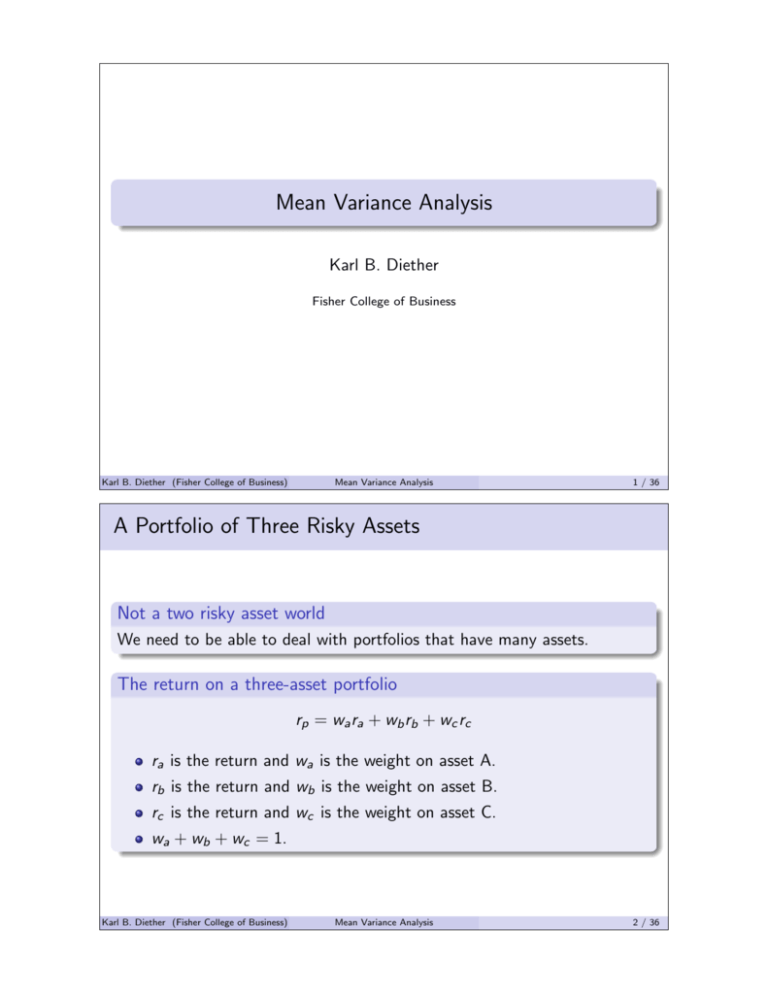
Mean Variance Analysis
Karl B. Diether
Fisher College of Business
Karl B. Diether (Fisher College of Business)
Mean Variance Analysis
1 / 36
A Portfolio of Three Risky Assets
Not a two risky asset world
We need to be able to deal with portfolios that have many assets.
The return on a three-asset portfolio
rp = wa ra + wb rb + wc rc
ra is the return and wa is the weight on asset A.
rb is the return and wb is the weight on asset B.
rc is the return and wc is the weight on asset C.
wa + wb + wc = 1.
Karl B. Diether (Fisher College of Business)
Mean Variance Analysis
2 / 36
A Portfolio of Three Risky Assets
Three asset portfolio: E (rp ) and σ(rp )
If A, B, and C are assets, wa , wb , and wc are the portfolio weights on each
asset, and wa + wb + wc = 1, then the expected return of the portfolio is
E (rp ) = wa E (ra ) + wb E (rb ) + wc E (rc )
the variance of the portfolio is
σ 2 (rp ) = wa2 σ 2 (ra ) + wb2 σ 2 (rb ) + wc2 σ 2 (rc )
+ 2wa wb cov(ra , rb ) + 2wa wc cov(ra , rc )
+ 2wb wc cov(rb , rc ),
and the standard deviation of the portfolio is
q
σ(rp ) = σ 2 (rp ).
Karl B. Diether (Fisher College of Business)
Mean Variance Analysis
3 / 36
A Portfolio of Three Risky Assets
Expected returns
The expected return of a portfolio is just a weighted sum of the individual
security expected returns.
Variance is a bit more complicated
Covariances are more influential than with a 2-asset portfolio.
Three covariances now instead of one.
As we add more assets, covariances become a more important
determinate of the portfolio’s variance (diversification).
Karl B. Diether (Fisher College of Business)
Mean Variance Analysis
4 / 36
Example: Three Risky Assets
You hate Microsoft so you invest in three competitors
Apple
Sun Micro
Red Hat
E (ri )
0.20
0.12
0.15
Apple
0.09
0.045
0.05
Covariance Matrix
Sun Micro
0.045
0.07
0.04
Red Hat
0.05
0.04
0.06
The covaraince matrix
The diagonal of the covariance matrix holds variances.
cov(rapple , rapple ) = σ 2 (rapple )
The covariance matrix is symmetric (row 1, column 2 = row 2, column 1):
cov(rapple , rsun ) = cov(rsun , rapple )
Karl B. Diether (Fisher College of Business)
Mean Variance Analysis
5 / 36
Example: Three Risky Assets
Computing E (rp ) and σ(rp )
E (rp ) = wa E (ra ) + ws E (rs ) + wh E (rh )
= 31 (0.2) + 13 (0.12) + 13 (0.15) = 15.7%
σ 2 (rp ) = wa2 σ 2 (ra ) + ws2 σ 2 (rs ) + wh2 σ 2 (rh )
+ 2wa ws cov(ra , rs ) + 2wa wh cov(ra , rh )
+ 2ws wh cov(rs , rh )
= 19 (0.09) + 19 (0.07) + 19 (0.06)
+ 2( 31 13 )(0.045) + 2( 31 13 )(0.05) + 2( 31 13 )(0.04)
= 0.0544
√
σ(rp ) = 0.0544 = 23.3%
Karl B. Diether (Fisher College of Business)
Mean Variance Analysis
6 / 36
A Portfolio of Many Risky Assets
An N asset portfolio
Consider a portfolio that has n assets (n can be a very large number like
1000, 7000, or even more than that).
The return on an N asset portfolio
rp = w1 r1 + w2 r2 + · · · + wn rn
n
X
=
wi ri
i=1
ri is the return on the ith asset in the portfolio.
wi is the portfolio weight for the ith asset.
P
The sum of the weights equals one: ni=1 wi = 1
Karl B. Diether (Fisher College of Business)
Mean Variance Analysis
7 / 36
Many Risky Assets: Expected Return
Expected return still a weighted sum
The expected return is a weighted average of the expected returns of the
individual securities in the portfolio:
E (rp ) = E w1 r1 + w2 r2 + · · · + wn rn
= w1 E (r1 ) + w2 E (r2 ) + · · · + wn E (rn )
n
X
=
wi E (ri )
i=1
Karl B. Diether (Fisher College of Business)
Mean Variance Analysis
8 / 36
Many Risky Assets: Variance
The variance
σr2p = w12 σ 2 (r1 ) + w22 σ 2 (r2 ) + · · · + wn2 σ 2 (rn )
+ 2w1 w2 cov(r1 , r2 ) + 2w1 w3 cov(r1 , r3 ) + · · · + 2w1 wn cov(r1 , rn )
+ 2w2 w3 cov(r2 , r3 ) + 2w2 w4 cov(r2 , r4 ) + · · · + 2w2 wn cov(r2 , rn )
..
..
..
.
.
.
+ 2wn−2 wn−1 cov(rn−2 , rn−1 ) + 2wn−2 wn cov(rn−2 , rn )
+ 2wn−1 wn cov(rn−1 , rn )
Writing the variance more compactly
2
σ (rp ) =
n
X
wi2 σ 2 (ri )
i=1
Karl B. Diether (Fisher College of Business)
+
n X
n
X
2wi wj cov(ri , rj )
i=1 j=i+1
Mean Variance Analysis
9 / 36
Mean Variance Analysis
10 / 36
Thinking About Risk
Risky Securities
What makes a stock risky?
Risky Portfolios
What makes a portfolio risky?
Karl B. Diether (Fisher College of Business)
Many Risky Assets: Variance
The importance of covariances
If the number of securities is large (and the weights are small),
covariances become the most important determinant of a portfolio’s
variance.
For a n asset portfolio there are n(n − 1)/2 covariance terms, and n
variance terms.
For example, a portfolio of a 1000 stocks, has 1000 variance terms
and 499,950 unique covariance terms.
Compare that to a portfolio of two assets which has 2 variance terms,
and 1 covariance term.
Karl B. Diether (Fisher College of Business)
Mean Variance Analysis
11 / 36
The Power of One
How does an asset affect a portfolio’s variance?
Just find all the terms in the variance equation that involve the asset.
Let’s do it for asset 1.
w12 σ 2 (r1 ) + 2w1 w2 cov(r1 , r2 ) + · · · + 2w1 wn cov(r1 , rn )
The risk of security 1 in portfolio p
An asset’s influence on a portfolio’s variance primarily depends on
how it covaries with the other assets in the portfolio.
Thus, what matters is how an asset covaries with the portfolio. The
above expression almost equals,
w1 cov(r1 , rp )
Karl B. Diether (Fisher College of Business)
Mean Variance Analysis
12 / 36
Minimizing the Portfolio Variance
A small thought experiment
To illustrate the importance of covariances lets think about how we could
find the minimum variance portfolio.
Finding the portfolio with the smallest possible variance
1
Find two securities already in the portfolio with different covariances
with the portfolio.
2
Add a little weight to the security with a lower cov(ri , rp ), and
subtract a little from the security with the higher covariance.
3
The portfolio variance is a little lower. Repeat steps 1 and 2 until the
variance cannot be lowered anymore.
The variance of the portfolio will be minimized when all the securities have
the same covariance with the portfolio:
cov(r1 , rp ) = cov(r2 , rp ) = · · · = cov(rn , rp )
Karl B. Diether (Fisher College of Business)
Mean Variance Analysis
13 / 36
Mean Variance Analysis
Asset allocation with many assets
Suppose you can invest in many risky assets. What is the optimal
allocation?
Clearly it depends on preferences.
Can we say anything about the portfolios that should be chosen?
What properity will the optimal or best portfolios have?
What does the investment opportunity set look like when we have
many assets?
Karl B. Diether (Fisher College of Business)
Mean Variance Analysis
14 / 36
Investment Opportunity Set
Red curve called the
efficient frontier
E(r)
Any point on the curve or to the
right is a feasible portfolio.
Feasible investment set is an area.
Global Min. Variance portfolio
σ(r)
Karl B. Diether (Fisher College of Business)
Mean Variance Analysis
15 / 36
The Investment Opportunity Set
The investment opportunity set
When there are many risky assets the feasible investment set is a curve
and the area to the right of the curve.
The boundary and the frontier
The curve in the graph is called the mean-variance boundary or the
mean-variance frontier.
The portion of the curve above the global minimum variance portfolio
is called the mean-variance efficient frontier or just the efficient
frontier.
An investor will only choose a portfolio on the efficient frontier.
Portfolios on the efficient frontier are called mean variance efficient
portfolios or efficient portfolios.
Adding more assets pushes the curve towards the Northwest corner of
the graph.
Karl B. Diether (Fisher College of Business)
Mean Variance Analysis
16 / 36
E(r)
Mean Variance Frontier: Adding Assets
σ(r)
Karl B. Diether (Fisher College of Business)
Mean Variance Analysis
17 / 36
The Mean Variance Boundary
How is the mean-variance boundary formed?
We pick the expected return we want, and then choose the weights of the
portfolio so that the variance of the portfolio is minimized.
Karl B. Diether (Fisher College of Business)
Mean Variance Analysis
18 / 36
Two-Fund Seperation
Two-Fund Separation
The entire mean-variance boundary can be created from any two
portfolios on the mean-variance boundary.
The entire efficient frontier can be created from any two mean
variance efficient portfolios.
More implications
A portfolio of portfolios on the mean-variance boundary will also be
on the boundary.
A portfolio of mean variance efficient portfolios will be on the efficient
frontier if the weight on each portfolio is positive.
Karl B. Diether (Fisher College of Business)
Mean Variance Analysis
19 / 36
Adding a Riskless Asset
How do you allocate your money between a riskless asset and risky
mean variance efficient portfolios?
Logically, this is the same as when we only had two risky assets.
We can draw a CAL between every efficient portfolio (the only ones
we care about) and the riskfree asset.
The best or optimal CAL is the one with the highest slope.
The optimal risky portfolio is the portfolio that is tangent to the
optimal CAL (the tangency portfolio).
Karl B. Diether (Fisher College of Business)
Mean Variance Analysis
20 / 36
Risk Free Asset and Many Risky Assets
CAL 3
E(r)
CAL 2
CAL 1
riskfree rate
σ(r)
Karl B. Diether (Fisher College of Business)
Mean Variance Analysis
21 / 36
E(r)
The Optimal CAL
The tangency portfolio
riskfree rate
σ(r)
Karl B. Diether (Fisher College of Business)
Mean Variance Analysis
22 / 36
The Optimal CAL
The optimal CAL: Definition
The CAL with the highest slope (Sharpe ratio):
Slope =
E (rp ) − rf
σ(rp )
The tangency portfolio
The optimal CAL is the tangency line between the riskfree rate and
the mean variance efficient frontier comprised entirely of risky assets.
The tangency portfolio is the portfolio – comprised of only risky
assets – with the highest Sharpe ratio.
Karl B. Diether (Fisher College of Business)
Mean Variance Analysis
23 / 36
The New Efficient Frontier
The new efficient frontier is the optimal CAL
If there are many risky assets and a riskfree asset, the efficient frontier is
the optimal CAL.
Optimal Allocations
Investors combine the tangency portfolio with the riskfree asset to
form their overall portfolio.
The allocation they choose depends on their preferences for risk and
expected return.
Note: Two-fund separation still holds; we can trace out the entire
frontier with two portfolios on the frontier.
I
For example, the tangency portfolio and the riskfree asset.
Karl B. Diether (Fisher College of Business)
Mean Variance Analysis
24 / 36
E(r)
The Optimal CAL
The tangency portfolio
riskfree rate
σ(r)
Karl B. Diether (Fisher College of Business)
Mean Variance Analysis
25 / 36
Finding the Tangency Portfolio
How do we find the tangency portfolio?
It is the portfolio – comprised of only risky assets – with the highest
Sharpe ratio:
E (rp ) − rf
SR =
σ(rp )
An inccorect method
1
Form a portfolio using all the risky securities (any portfolio will do).
2
Find two securities already in the portfolio with different Sharpe
ratios.
Wrong! Step 2 is not quite right. Let’s think about the goal.
Karl B. Diether (Fisher College of Business)
Mean Variance Analysis
26 / 36
Finding the Tangency Portfolio
What we care about
We only care about how a security affects the portfolio’s Sharpe ratio.
Remember, securities only affect the variance of a portfolio via its
covariance with the portfolio.
Examine the marginal sharpe ratios
We really just need to look for securities with different,
E (ri ) − rf
cov(ri , rp )
Note: the above ratio is called the marginal Sharpe ratio.
Karl B. Diether (Fisher College of Business)
Mean Variance Analysis
27 / 36
Finding the Tangency Portfolio
The correct method
1
Form a portfolio using all the risky securities (any portfolio will work).
2
Find two securities already in the portfolio with different risk premium
to covariance ratios:
E (ri ) − rf
cov(ri , rp )
3
Add a little weight to the security with a higher ratio, and subtract a
little from the security with the lower ratio.
4
Keep repeating steps 1 – 3 until, marginal Sharpe ratios are equal
across all securities.
Karl B. Diether (Fisher College of Business)
Mean Variance Analysis
28 / 36
Finding the Tangency Portfolio
All the marginal Sharpe ratios are equal
For the tangency portfolio (T), the following is true:
E (r1 ) − rf
E (r2 ) − rf
E (rn ) − rf
=
= ··· =
cov(r1 , rT )
cov(r2 , rT )
cov(rn , rT )
This includes all individual securities and other portfolios.
Rewriting compactly
We can write the tangency condition as the following:
E (rj ) − rf
E (ri ) − rf
=
cov(ri , rT )
cov(rj , rT )
Karl B. Diether (Fisher College of Business)
for all i and j
Mean Variance Analysis
29 / 36
Example: The Tangency Portfolio
Suppose you can invest in two risky assets and a riskfree asset
E(r)
11%
16%
6%
Stock 1
Stock 2
Riskfree
σ
20%
25%
cov(r1 , r2 ) = 0.025
The tangency condition
Remember, the following is true for the tangency portfolio (T):
E (r1 ) − rf
E (r2 ) − rf
=
cov(r1 , rT )
cov(r2 , rT )
Karl B. Diether (Fisher College of Business)
Mean Variance Analysis
30 / 36
Example: The Tangency Portfolio
Computing covariance of a security with a portfolio
If x, y , and z are random variables and A and B are constants,
cov(z, Ax + By ) = A cov(z, x) + B cov(z, y )
If portfolio P is comprised of two assets called A and B, w is the weight on
A and 1 − w is the weight on B, then the covariance of a security I with
portfolio P is the following:
cov(ri , rp ) = w cov(ri , ra ) + (1 − w ) cov(ri , rb )
Karl B. Diether (Fisher College of Business)
Mean Variance Analysis
31 / 36
Example: The Tangency Portfolio
The rule applied to the example
cov(r1 , rT ) = w cov(r1 , r1 ) + (1 − w ) cov(r1 , r2 )
= w σ 2 (r1 ) + (1 − w ) cov(r1 , r2 )
cov(r2 , rT ) = w cov(r2 , r1 ) + (1 − w ) cov(r2 , r2 )
= w cov(r1 , r2 ) + (1 − w )σ 2 (r2 )
Now we are ready to find the tangency portfolio
We can solve for the optimal w by using the tangency portfolio condition:
E (r1 ) − rf
E (r2 ) − rf
=
cov (r1 , rT )
cov (r2 , rT )
Karl B. Diether (Fisher College of Business)
Mean Variance Analysis
32 / 36
Example: The Tangency Portfolio
E (r1 ) − rf
E (r2 ) − rf
=
cov (r1 , rT )
cov (r2 , rT )
E (r1 ) − rf cov (r2 , rT ) = E (r2 ) − rf cov (r1 , rT )
5 wcov (r1 , r2 ) + (1 − w )σ 2 (r2 ) = 10 w σ 2 (r1 ) + (1 − w )cov (r1 , r2 )
5[0.025w + (1 − w )0.0625] = 10[0.04w + (1 − w )0.025]
5[−0.0375w + 0.0625] = 10[0.015w + 0.025]
−0.1875w + 0.3125 = 0.15w + 0.25
0.3375w = 0.0625
w = 0.185
The optimal portfolio is 18.5% in stock 1 and 81.5% in stock 2.
Karl B. Diether (Fisher College of Business)
Mean Variance Analysis
33 / 36
Example: The Tangency Portfolio
What is the Sharpe Ratio of the tangency portfolio?
E (rT ) = 0.185(0.11) + 0.815(0.16) = 15.08%
σ 2 (rt ) = 0.1852 (0.22 ) + 0.8152 (0.252 ) + 2(0.185)(0.815)(0.025)
= 0.05
SRT =
0.1508 − 0.06
√
= 0.406
0.05
Compare that to the Sharpe ratios of stock 1 and 2:
0.11 − 0.06
= 0.25
0.20
0.16 − 0.06
SR2 =
= 0.40
0.25
SR1 =
Karl B. Diether (Fisher College of Business)
Mean Variance Analysis
34 / 36
A Few Things to Think About
Problems with mean variance analysis
Can you think of any limitations with respect to mean variance
analysis?
What are some of the practical problems people face when they try to
use mean variance analysis?
How might people manage some of these practical problems?
Warren Buffet
Warren Buffet claims he doesn’t engage in mean variance analysis.
Is that a mistake or can you think of reasons why it doesn’t make
sense for him to use mean variance analysis?
Karl B. Diether (Fisher College of Business)
Mean Variance Analysis
35 / 36
Summary
An asset’s influence on a portfolio’s variance primarily depends on
how it covaries with the other assets in the portfolio.
A rational and risk averse investor will only invest in efficient
portfolios.
Efficient portfolios have the highest expected return for a given
standard deviation
If there is a risk free asset then the efficient frontier is a CAL line
between the riskfree asset and the tangency portfolio.
The tangency portfolio is composed of only risky assets.
The tangency portfolio has the highest Sharpe ratio of any portfolio
composed of risky assets.
In the tangency portfolio all the marginal Sharpe ratios are equal.
Karl B. Diether (Fisher College of Business)
Mean Variance Analysis
36 / 36