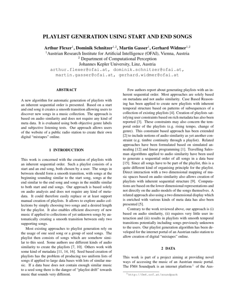
PLAYLIST GENERATION USING START AND END SONGS
Arthur Flexer1 , Dominik Schnitzer1,2 , Martin Gasser1 , Gerhard Widmer1,2
1
Austrian Research Institute for Artificial Intelligence (OFAI), Vienna, Austria
2
Department of Computational Perception
Johannes Kepler University, Linz, Austria
arthur.flexer@ofai.at, dominik.schnitzer@ofai.at,
martin.gasser@ofai.at, gerhard.widmer@ofai.at
ABSTRACT
A new algorithm for automatic generation of playlists with
an inherent sequential order is presented. Based on a start
and end song it creates a smooth transition allowing users to
discover new songs in a music collection. The approach is
based on audio similarity and does not require any kind of
meta data. It is evaluated using both objective genre labels
and subjective listening tests. Our approach allows users
of the website of a public radio station to create their own
digital “mixtapes” online.
1 INTRODUCTION
This work is concerned with the creation of playlists with
an inherent sequential order. Such a playlist consists of a
start and an end song, both chosen by a user. The songs in
between should form a smooth transition, with songs at the
beginning sounding similar to the start song, songs at the
end similar to the end song and songs in the middle similar
to both start and end songs. Our approach is based solely
on audio analysis and does not require any kind of metadata. It could therefore easily replace or at least support
manual creation of playlists. It allows to explore audio collections by simply choosing two songs and a desired length
for the playlist. It also enables efficient discovery of new
music if applied to collections of yet unknown songs by automatically creating a smooth transition between only two
supporting songs.
Most existing approaches to playlist generation rely on
the usage of one seed song or a group of seed songs. The
playlist then consists of songs which are somehow similar to this seed. Some authors use different kinds of audio
similarity to create the playlists [7, 10]. Others work with
some kind of metadata [11, 14, 16]. Seed based creation of
playlists has the problem of producing too uniform lists of
songs if applied to large data bases with lots of similar music. If a data base does not contain enough similar music
to a seed song there is the danger of “playlist drift” towards
music that sounds very different.
Few authors report about generating playlists with an inherent sequential order. Most approaches are solely based
on metadata and not audio similarity. Case Based Reasoning has been applied to create new playlists with inherent
temporal structure based on patterns of subsequences of a
collection of existing playlists [4]. Creation of playlists satisfying user constraints based on rich metadata has also been
reported [3]. These constraints may also concern the temporal order of the playlists (e.g. rising tempo, change of
genre). This constraint based approach has been extended
[2] to include notions of audio similarity as yet another constraint (e.g. timbre continuity through a playlist). Related
approaches have been formulated based on simulated annealing [12] and linear programming [1]. Travelling Salesman algorithms applied to audio similarity have been used
to generate a sequential order of all songs in a data base
[15]. Since all songs have to be part of the playlist, this is a
quite different kind of organising principle for the playlist.
Direct interaction with a two dimensional mapping of music spaces based on audio similarity also allows creation of
playlists with inherent sequential structure [9]. Computations are based on the lower dimensional representations and
not directly on the audio models of the songs themselves. A
related approach also using a two dimensional display which
is enriched with various kinds of meta data has also been
presented [5].
Contrary to the work reviewed above, our approach is (i)
based on audio similarity, (ii) requires very little user interaction and (iii) results in playlists with smooth temporal
transitions potentially including songs previously unknown
to the users. Our playlist generation algorithm has been developed for the internet portal of an Austrian radio station to
allow creation of digital “mixtapes” online.
2 DATA
This work is part of a project aiming at providing novel
ways of accessing the music of an Austrian music portal.
The FM4 Soundpark is an internet platform 1 of the Aus1
http://fm4.orf.at/soundpark
No.
%
HiHo
226
9
Regg
60
2
Funk
56
2
Elec
918
36
Pop
158
6
Rock
1148
45
Table 1. Number of songs and percentages across genres
in our data base. Genres are Hip Hop, Reggae, Funk, Electronic, Pop and Rock.
trian public radio station FM4. This internet platform allows
artists to present their music free of any cost in the WWW.
All interested parties can download this music free of any
charge. At the moment this music collection contains about
10000 songs but it is only organised alphabetically and in
a coarse genre taxonomy. The artists themselves choose
which of the six genre labels “Hip Hop, Reggae, Funk, Electronic, Pop and Rock” best describe their music. We use a
development data base of 2566 songs for our experiments.
Number of songs and percentages across genres are given in
Tab. 1. The distribution of genres is quite unbalanced with
“Electronic” and “Rock” together taking up 81%. This is
representative of the full data base.
From the 22050Hz mono audio signals two minutes from
the center of each song are used for further analysis. We divide the raw audio data into non-overlapping frames of short
duration and use Mel Frequency Cepstrum Coefficients
(MFCC) to represent the spectrum of each frame. MFCCs
are a perceptually meaningful and spectrally smoothed representation of audio signals. MFCCs are now a standard
technique for computation of spectral similarity in music
analysis (see e.g. [6]). The frame size for computation of
MFCCs for our experiments was 46.4ms (1024 samples).
We used the first 20 MFCCs for all our experiments.
3 METHODS
3. compute a similarity matrix between all songs using
the Kullback-Leibler divergence between respective
G1 models
We use one single Gaussian (G1) with full covariance to
represent the MFCCs of each song [8]. For single Gaussians, p(x) = N (x; µp , σp ) and q(x) = N (x; µq , σq ), there
is a closed form of the Kullback-Leibler divergence [13]:
KLN (pkq) = 0.5 log
det (Σp )
det (Σq )
+ 0.5T r Σ−1
p Σq
0
+ 0.5 (µp − µq ) Σ−1
p (µq − µp ) −
d
2
(1)
where T r(M ) denotes the trace of the matrix M , T r(M ) =
Σi=1..n mi,i . Dropping constants and symmetrizing the divergence yields the following approximation [17]:
−1
DKL (p, q) = T r Σ−1
p Σq + T r Σq Σp
0
−1
+ T r Σ−1
(µp − µq ) (µq − µp )
p + Σq
(2)
Please note that this approximation is symmetric, i.e.
DKL (p, q) = DKL (q, p), and that the self-similarity is
non-zero, i.e. DKL (p, p) 6= 0. Actually, DKL (p, p) =
2d with d being the dimensionality of the data vectors (20
MFCCs in our case).
3.2 Computing playlists
Our algorithm for computation of a playlist of length p (excluding start and end song) for a database of n songs Si ,
starting at song Ss and ending at song Se consists of the
following steps:
Our playlist generation algorithm consists of two basic parts:
(i) computation of similarities between songs, (ii) computation of the actual playlists based on these similarities. Please
note that the actual generation of playlists does not rely on a
specific similarity function and could therefore also be done
using different approaches towards computation of similarity.
1. for all i = 1, ..., n songs compute the divergences to
the start song DKL (i, s) and the end song DKL (i, e)
3.1 Computing spectral similarity of songs
3. for all i = 1, ..., m songs compute a divergence ratio:
We use the following approach to music similarity based on
spectral similarity. For a given music collection of songs, it
consists of the following steps:
1. for each song, compute MFCCs for short overlapping
frames as described in Sec. 2
2. find the d% songs with greatest divergence DKL (i, s)
to the start song Ss ; find the d% songs with greatest
divergence DKL (i, e) to the end song Se ; discard all
songs which are in both of these groups; keep remaining m songs for further processing
R(i) =
(3)
4. compute step width for playlist:
step =
2. train a single Gaussian (G1) to model each of the songs
DKL (i, s)
DKL (i, e)
R(s) − R(e)
p+1
(4)
5. compute p ideal positions (i.e. ideal divergence ratios)
R̂(j), j = 1, ..., p :
R̂(j) = R(s) + j ∗ step
(5)
6. select the p real songs Sj that best match the ideal
divergence ratios R̂(j), j = 1, ..., p :
Sj = arg min |R̂(j) − R(i)|
i=1,...,m
(6)
The main part of our algorithm is the computation of divergence ratios R(i). Songs which are closer to the start
song Ss than to the end song Se will have a divergence ratio
R(i) < 1. Songs which are closer to the end song Se than
to the start song Ss will have a divergence ratio R(i) > 1.
Songs which have about the same divergence to both songs
will have a divergence ratio R(i) around 1. Songs which
have a big divergence to both start and end song will therefore also have a divergence ratio R(i) around 1 and therefore
might end up as part of the middle section of a playlist. This
is of course not as desired since only songs which are close
to either or both the start and end song should be part of the
playlist. Songs too distant from both start and end song appear as outliers to the listeners. Therefore we discard songs
which are distant to both start and end song during step 2
of the above algorithm. The amount of songs we discard is
controlled with the parameter d. In initial experiments we
found out that d = 95% works well for this data set.
The playlist is then computed in the divergence ratio space:
R(s) serves as the starting position and R(e) as the end position of the list. The aim is to find p songs which are at
equally spaced positions between these start and end positions. This is done by computing a step width in step 4 of the
algorithm, computing ideal positions for the playlist songs
in the divergence ratio space in step 5 and finally finding
songs that best match these ideal positions in step 6.
4 RESULTS
4.1 Objective evaluation
One possibility to achieve an objective evaluation is to use
the genre labels as indicators of music similarity. For a
playlist with start song belonging to genre A and end song
belonging to genre B we formulate the following hypotheses:
• the playlist should contain mostly songs from genres
A and B
• at the beginning of the playlist, most songs should be
from genre A, at the end from genre B and from both
genres in the middle
t
r
u
e
HiHo
Regg
Funk
Elec
Pop
Rock
HiHo
73
35
20
13
22
4
nearest neighbour classification
Regg Funk Elec Pop Rock
8
0
11
4
4
33
2
13
5
12
5
29
16
13
18
7
3
56
8
13
3
4
13
26
32
1
1
3
4
87
Table 2. Confusion matrix of genre classification results
(nearest neighbour classification vs. true genre label). Results are given in percentages separately per genre in each
row. Genres are Hip Hop, Reggae, Funk, Electronic, Pop
and Rock.
The success of such an approach depends strongly on
how well the genre labels actually indicate music similarity.
This can be measured by looking at the genre classification
results. Table 2 gives a confusion matrix for a 10-fold crossvalidation experiment with one-nearest neighbour classification using the divergences DKL . Results are given in
percentages separately per genre in each row. Some of the
genres can be classified very well (Hip Hop: 73%, Rock:
87%), others somewhat well (Electronic: 56%) and some
quite badly (Reggae, Funk and Pop are all around 30%).
Consequently, any playlist evaluation relying on the genre
information should do quite well on genres Hip Hop, Rock
and maybe Electronic. But it would show the same confusion of labels for all other genres.
We randomly chose 50 songs from each of the six genres as candidates for start and end songs. Since our playlist
algorithm gives identical members of playlists in reversed
order when start and end songs are exchanged, we need to
look at only (6 × (6 − 1))/2 = 15 possible combinations
of our six genres. For each combination of two genres A
and B, we compute all possible 50 × 50 playlists using the
candidate songs as start and end songs. This yields 37500
playlists altogether. The length of each playlist is nine songs
excluding start and end songs. We divide all playlists in
three sections (first, middle and last three songs) and report
distribution of songs across genres in the playlists. Instead
of showing results for all possible 15 combinations of genres we concentrate on a number of examples showing the
range of quality one can expect.
Table 3 shows the results for playlists starting at Hip Hop
and ending at Rock. Both genres dominate (33% and 38%)
the beginning of the playlists (Sec1). Whereas Hip Hop
quickly diminishes to 5% and 2%, Rock rises to 81% and
88% at the end.
The results for playlists starting at Hip Hop and ending
at Electronic (Tab. 4) as well as for playlists starting at Electronic and ending at Rock (Tab. 5) work equally well. The
respective genres dominate the beginning of the playlists.
Sec1
Sec2
Sec3
HiHo
33
5
2
Regg
5
1
0
Funk
2
2
3
Elec
15
7
4
Pop
8
4
2
Rock
38
81
88
Table 3. Distribution of songs across genres in playlists
starting at Hip Hop and ending at Rock. Results given for
first, middle and last section of playlists (Sec1 to Sec3).
Sec1
Sec2
Sec3
HiHo
30
6
2
Regg
5
2
2
Funk
2
3
3
Elec
35
66
70
Pop
8
5
4
Sec1
Sec2
Sec3
HiHo
26
6
3
Regg
7
1
0
Funk
2
2
2
Elec
20
7
4
Pop
7
4
2
Rock
38
80
88
Table 6. Distribution of songs across genres in playlists
starting at Reggae and ending at Rock. Results given for
first, middle and last section of playlists (Sec1 to Sec3).
Rock
19
18
18
Sec1
Sec2
Sec3
HiHo
19
17
12
Regg
3
4
3
Funk
8
4
4
Elec
28
20
22
Pop
13
19
16
Rock
29
36
42
Table 4. Distribution of songs across genres in playlists
starting at Hip Hop and ending at Electronic. Results given
for first, middle and last section of playlists (Sec1 to Sec3).
Table 7. Distribution of songs across genres in playlists
starting at Funk and ending at Pop. Results given for first,
middle and last section of playlists (Sec1 to Sec3).
The start genres diminish quickly and the end genres are
most prominent in the last sections (Sec3). Tables 3 to 5
give results for the three genres which also achieve the best
classification results (see Tab. 2). The results are basically in
line with the two hypotheses we formulated at the beginning
of this section. Only the fact that the end genre is already
very prominent at the beginning of the playlists (Sec1) is a
bit surprising. This might be due to the fact that the end genres in Tables 3 to 5 are also the most numerous in our data
base (Electronic 36% and Rock 45% of all songs in the data
base, see Tab. 1).
Table 6 shows the results for playlists starting at Reggae
and ending at Rock. The amount of songs from genre Rock
rises from 38% to 80% to 88% going from Sec1 to Sec3 as
expected. Genre Reggae is somewhat under-represented in
all sections of the playlists. Going back to the genre classification confusion matrix in Tab. 2, it is clear that there is a
lot of mix-up between genres Reggae and Hip Hop. Consequently, Tab. 6 shows a considerable amount of Hip Hop in
Sec1, diminishing towards Sec3.
The results for playlists starting at Funk and ending at
Pop given in Tab. 7 are even less satisfactory. The genre
classification confusion matrix in Tab. 2 shows that genre
Funk is confused with almost all other genres and genre
Pop strongly with genre Rock. As a result, the only visible trend in Tab. 7 is a rising amount of songs from genres
Pop and Rock going from Sec1 to Sec3. This clearly indicates the limits of our approach to objective evaluation of
playlist generation. Such an evaluation only makes sense
with reliable genre label information.
The amount of songs which are being excluded from becoming members of the playlist because of being too dissimilar from both start and end song was set to d = 95% for
all experiments (see step 2 in Sec. 3.2). Relaxing this constraint to smaller values leads to less clear distribution of
genres (i.e. less songs in the playlists have the same genre
label as the start and end songs).
Sec1
Sec2
Sec3
HiHo
13
8
5
Regg
3
2
1
Funk
2
2
3
Elec
42
8
3
Pop
6
5
3
Rock
34
77
85
Table 5. Distribution of songs across genres in playlists
starting at Electronic and ending at Rock. Results given for
first, middle and last section of playlists (Sec1 to Sec3).
4.2 Subjective evaluation
Our playlist generation algorithm can be utilised by users
of the FM4 Soundpark website 2 to create their own digital
“mixtapes” online. Therefore the best evaluation would be
a user study with people actually using this service on the
internet. Such a user study is planned for the future. During
the development phase of the project, we decided to do an
internal form of user study by having one of the authors listen to a number of playlists and judge their quality. This one
person has considerable experience with popular music for
having been a record collector and DJ for about two decades.
While this approach has the problem of being highly subjective it does have the advantage of actually judging the “raw”
playlists instead of a certain implementation and user interface.
As pointed out in Sec. 4.1, our playlist algorithm gives
identical members of playlists in reversed order when start
2
http://fm4.orf.at/soundpark
and end songs are exchanged. Therefore, we look at only
(6 × (6 − 1))/2 = 15 possible combinations of our six genres (see two leftmost columns in Tab. 8). For each combination of two genres A and B, we randomly choose three
of the 50 × 50 playlists computed as described in Sec. 4.1.
This gives 45 playlists for evaluation. Our evaluator listened
to all the playlists using the “XMMS 1.2.10 - Cross platform multimedia player” 3 . He would first listen to the start
song, then the end song and then the songs in between in
the correct order. The evaluator was allowed to freely move
through a song by skipping parts and moving back and forth
in time. He was also allowed to re-listen to songs in the
playlist if necessary.
For each playlist, the evaluator was asked to answer the
following two questions which are tightly connected to our
two hypotheses formulated in Sec. 4.1:
• How many outliers are in the playlist which do not fit
the overall flavour of the playlist?
• Is the order of songs in the playlist from the start to
the end song apparent?
The first question should allow to judge whether all the
songs in a playlist really are similar to either the start or the
end song, or are located somewhere in the intended middle.
The second question aims at the sequential ordering of the
songs. Songs at the beginning should be more similar to the
start song, songs at the end to the end song. The second
question can be answered with either “yes”, “somewhat” or
“no”.
The results of the evaluation are given in Tab. 8. For
each combination of genres, the average number of outliers
is given (average taken over three playlists). It is also indicated how the second question has been answered for the
three playlists of a certain combination of genres. Each “x”
in a column stands for the respective answer given for one
playlist. So for each row (i.e. combination of genres) three
“x” indicate three answers to the second question. At the
bottom row, the average number of outliers is given as well
as the percentages of different answers to the question about
the sequential order of the playlists is given.
The average number of outliers in a playlist is quite low
at 1.1 out of possible 9. This means that on average, a user
might want to delete one song from an automatically created playlist. While for a lot of combinations of genres this
number is 0 and therefore perfect, for some genre combinations the number of outliers is quite high. E.g. for playlists
starting at Hip Hop and ending at Reggae, an average of 4.7
songs are rated as outliers. The reasons seems to be that
for a listener, the defining part of a Reggae song is the offbeat percussion which is not well conserved in our timbral
representation of music. Instead, the rhythm guitar seems
3
http://www.xmms.org
Genres
from to
HiHo Regg
HiHo Funk
HiHo Elec
HiHo Pop
HiHo Rock
Regg Funk
Regg Elec
Regg Pop
Regg Rock
Funk Elec
Funk Pop
Funk Rock
Elec
Pop
Elec
Rock
Pop
Rock
average
# of
outliers
4.7
1.7
1.3
2.7
0
0.7
1.3
1.3
0.3
1.0
1.7
0
0
0
0
1.1
yes
xx
xxx
xxx
xx
xxx
xxx
xx
xx
xx
xx
xxx
xx
xxx
71.1%
order apparent
somewhat
x
x
no
xx
xx
x
x
x
x
x
x
x
17.8%
11.1%
Table 8. Results of the subjective evaluation. For each combination of genres, the average number of outliers and the
answers to the question concerning the order in the playlist
is given. At the bottom row, average number of outliers as
well as the percentages of different answers to the question
about order are given.
to dominate the models giving rise to high similarities with
certain types of rock songs. Other sources of mistakes are
recordings of poor acoustic quality which are found to be
similar to each other no matter what the genres of the songs
are. The sequential order of the playlists seems to work
very well with it being apparent in 71% of all playlists and
“somewhat” apparent in another 17.8%. One problem with
the sequential ordering that we noticed is a kind of “tilting”effect at the middle of playlists: the first half would be very
close to the start song, the second half to the end song but
a sort of smooth transition is missing. This was sometimes
the case if start and end songs are very different and the data
base might not even contain songs fitting in between. Another problem are too many outliers obscuring the overall
order of a playlist.
As with the objective evaluation in Sec. 4.1, relaxing the
amount of songs which are being excluded from becoming
members of the playlist below d = 95% (see step 2 in Sec.
3.2) results in more outliers and less clear sequential order
of the playlists.
5 CONCLUSION
We have presented a new approach for the generation of
playlists using start and end songs and showing inherent sequential order. Our approach is based on audio similarity
and requires very little user interaction. Both objective evaluation based on genre labels of songs and subjective evaluation based on listening tests showed that the concept works
well.
Our playlist generation algorithm can be utilised by users
of the website of a public radio station to create their own
digital “mixtapes” online. Since our evaluation showed that,
on average, at least one song does not fit the overall playlist,
an editing functionality might be added to the user interface.
[8] Mandel M.I., Ellis D.P.W.: Song-Level Features and
Support Vector Machines for Music Classification, Proceedings of the 6th International Conference on Music Information Retrieval (ISMIR’05), London, UK,
September 11-15, 2005.
[9] Neumayer R., Dittenbach M., Rauber A.: PlaySOM
and PocketSOMPlayer: Alternative Interfaces to Large
Music Collections, Proceedings of the 6th International
Conference on Music Information Retrieval (ISMIR’05),
London, UK, September 11-15, pp. 618-623, 2005.
6 ACKNOWLEDGEMENTS
[10] Pampalk E., Pohle T., Widmer G.: Dynamic Playlist
Generation Based on Skipping Behaviour, Proceedings
of the 6th International Conference on Music Information Retrieval (ISMIR’05), London, UK, September 1115, 2005.
Parts of this work have been funded by the “Österreichische
Forschungsförderungsgesellschaft (FFG)” (Bridge-project
815474 and “Advanced Knowledge Technologies: Grounding, Fusion, Applications AKT:GFA”-project).
[11] Pauws S., Eggen B.: PATS: Realization and User Evaluation of an Automatic Playlist Generator, Proceedings of
the 3rd International Conference on Music Information
Retrieval (ISMIR’02), Paris, France, pp. 222-230, 2002.
7 REFERENCES
[1] Alghoniemy M., Tewfik A.: A network flow model for
playlist generation, IEEE International Conference on
Multimedia and Expo (ICME’01), 2001.
[2] Aucouturier J.-J., Pachet F.: Finding songs that sound
the same, Proceedings of IEEE Benelux Workshop on
Model based Processing and Coding of Audio, Leuven,
Belgium, Nov. 2002, 2002.
[3] Aucouturier J.-J., Pachet F.: Scaling up music playlist
generation, Proceedings of IEEE International Conference on Multimedia and Expo (ICME), Lausanne,
Switzerland, 2002.
[4] Baccigalupo C., Plaza E.: Case-Based Sequential Ordering of Songs for Playlist Recommendation, European Conference on Case Based Reasoning (ECCBR
’06), Lecture Notes in Computer Science, Springer
Berlin/Heidelberg, Volume 4106/2006, 2006.
[5] Gulik R., Vignoli F.: Visual Playlist Generation on the
Artist Map, Proceedings of the 6th International Conference on Music Information Retrieval (ISMIR’05), London, UK, 2005.
[6] Logan B.: Mel Frequency Cepstral Coefficients for Music Modeling, Proc. of the International Symposium on
Music Information Retrieval (ISMIR’00), 2000.
[7] Logan B.: Music Recommendation from Song Sets,
Proceedings of the 5th International Conference on Music Information Retrieval (ISMIR’04), Barcelona, Spain,
October 10-14, 2004.
[12] Pauws S., Verhaegh W., Vossen M.: Fast Generation of
Optimal Music Playlists using Local Search, Proceedings of the 7th International Conference on Music Information Retrieval (ISMIR’06), Victoria, Canada, 2006.
[13] Penny W.D.: Kullback-Liebler Divergences of Normal,
Gamma, Dirichlet and Wishart Densities, Wellcome Department of Cognitive Neurology, 2001.
[14] Platt J.C., Burges C.J.C., Swenson S., Weare C., Zheng
A.: Learning a Gaussian Process Prior for Automatically
Generating Music Playlists, Advances in Neural Information Processing Systems 14, pp. 1425-1432, 2002.
[15] Pohle T., Knees P., Schedl M., Pampalk E., Widmer G.:
”Reinventing The Wheel”: A Novel Approach to Music
Player Interfaces, IEEE Multimedia, 14(3), pp. 46-54,
2007.
[16] Ragno R., Burges C.J.C., Herley C.: Inferring Similarity Between Music Objects with Application to Playlist
Generation, Proc. 7th ACM SIGMM International Workshop on Multimedia Information Retrieval, 2005.
[17] Schnitzer D.: Mirage - High-Performance Music Similarity Computation and Automatic Playlist Generation,
Vienna University of Technology, Austria, Master Thesis, 2007.