1
CHAPTER 9
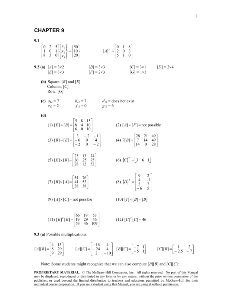
9.1
x  50 
0 2 5 
 1 
 
1 0 1  x 2   10 
8 3 0 
20 

 x3 
 
9.2 (a) [A] = 32
[E] = 33
0 1 8 
[ A]T  2 0 3
5 1 0
[B] = 33
[F] = 23
[C] = 31
[G] = 13
[D] = 24
(b) Square: [B] and [E]
Column: [C]
Row: [G]
(c) a12 = 7
e22 = 2
b23 = 7
f12 = 0
d32 = does not exist
g12 = 6
(d)
5 8 15 
(1) [ E ]  [ B ]  8 4 10 
6 0 10 
 3  2  1
4 
(3) [ B]  [ E ]    6 0
 2 0  2
(2) [ A]  [ F ]  not possible
28 21 49 
(4) 7[ B]   7 14 49 
14 0 28 
25 13 74 
(5) [ E ]  [ B]  36 25 75 
28 12 52 
(6) C  3 6 1
54 76 
(7) [ B]  [ A]   41 53 
28 38 
(8) D
(9) [ A]  [C ]  not possible
(10) [ I ]  [ B]  [ B]
66 19 53 
(11) [ E ]T [ E ]  19 29 46 
53 46 109 
(12) [C ]T [C ]  46
T
T
2
9
4

1


3
7
 6 5 
9.3 (a) Possible multiplications:
4 15 
[ A][ B ]  8 29 
9 29 
4 
  16
[ A][C ]   24
4  [ B][C ]   7 1
  5 1
 2
 10 
2
[C ][B]   1
 2.5  7
Note: Some students might recognize that we can also compute [B][B] and [C][C]:
PROPRIETARY MATERIAL. © The McGraw-Hill Companies, Inc. All rights reserved. No part of this Manual
may be displayed, reproduced or distributed in any form or by any means, without the prior written permission of the
publisher, or used beyond the limited distribution to teachers and educators permitted by McGraw-Hill for their
individual course preparation. If you are a student using this Manual, you are using it without permission.
2
[C ][C ]   10  6
 9 7 
[ B][ B]  2.5 9 
1.5 5.5
(b) [B][A] and [C][A] are impossible because the inner dimensions do not match:
(22) * (32)
(c) According to (a), [B][C]  [C][B]
9.4 The equations can be rearranged into a format for plotting x2 versus x1:
x 2  3  0.5 x1
x2 
34 1
 x1
6 6
10
8
6
4
2
0
0
2
4
6
8
10
Therefore, the solution is x1 = 4, x2 = 5. The results can be checked by substituting them back
into the original equations:
4(4)  8(5)  24
4  6(5)  34
9.5 (a) The equations can be rearranged into a format for plotting x2 versus x1:
x 2  12  0.11x1
x 2  10 
2
x1
17.4
PROPRIETARY MATERIAL. © The McGraw-Hill Companies, Inc. All rights reserved. No part of this Manual
may be displayed, reproduced or distributed in any form or by any means, without the prior written permission of the
publisher, or used beyond the limited distribution to teachers and educators permitted by McGraw-Hill for their
individual course preparation. If you are a student using this Manual, you are using it without permission.
3
120
100
80
60
40
20
0
0
200
400
600
800
If you zoom in, it appears that there is a root at about (404.6, 56.5).
56.6
56.55
56.5
56.45
56.4
404
404.5
405
405.5
The results can be checked by substituting them back into the original equations:
 1.1(404 .6)  10(56.5)  119 .94  120
 2(404 .6)  17.4(56.5)  173 .9  174
(b) The plot suggests that the system may be ill-conditioned because the slopes are so similar.
(c) The determinant can be computed as
D  1.1(17.4)  10(2)  0.86
which is relatively small. Note that if the system is normalized first by dividing each equation
by the largest coefficient,
 0.11x1  x 2  12
 0.11494 x1  x 2  10
the determinant is even smaller
D  0.11(1)  1(0.11494 )  0.00494
(d) Using Eqs. (9.10) and (9.11) yields
PROPRIETARY MATERIAL. © The McGraw-Hill Companies, Inc. All rights reserved. No part of this Manual
may be displayed, reproduced or distributed in any form or by any means, without the prior written permission of the
publisher, or used beyond the limited distribution to teachers and educators permitted by McGraw-Hill for their
individual course preparation. If you are a student using this Manual, you are using it without permission.
4
x1 
17.4(120)  10(174)
 404.6512
0.86
x2 
 1.1(174)  (2)(120)
 56.51163
0.86
9.6 (a) The determinant can be computed as:
A1  1 1  1(0)  1(1)  1
1 0
A2  2 1  2(0)  1(3)  3
3 0
A3  2 1  2(1)  1(3)  1
3 1
D  0(1)  2(3)  5(1)  1
(b) Cramer’s rule
x1 
x2 
x3 
9 2 5
9 1 1
10 1 0
D

6
6
1

8
 8
1

5
5
1
0 9 5
2 9 1
3 10 0
D
0 2 9
2 1 9
3 1 10
D
(c) The results can be checked by substituting them back into the original equations:
2(8)  5(5)  9
2(6)  (8)  5  9
3(6)  (8)  10
9.7 (a) The equations can be rearranged into a format for plotting x2 versus x1:
PROPRIETARY MATERIAL. © The McGraw-Hill Companies, Inc. All rights reserved. No part of this Manual
may be displayed, reproduced or distributed in any form or by any means, without the prior written permission of the
publisher, or used beyond the limited distribution to teachers and educators permitted by McGraw-Hill for their
individual course preparation. If you are a student using this Manual, you are using it without permission.
5
x 2  9.5  0.5 x1
x 2  9.4  0.51x1
14.6
14.55
14.5
14.45
14.4
9.8
9.9
10
10.1
10.2
The solution is x1 = 10, x2 = 14.5. Notice that the lines have very similar slopes.
(b) The determinant can be computed as
D  0.5(2)  (1)1.02  0.02
(c) The plot and the low value of the determinant both suggest that the system is illconditioned.
(d) Using Eqs. (9.10) and (9.11) yields
x1 
 9.5(2)  (1)(18.8)
 10
0.02
x2 
0.5(18.8)  (9.5)1.02
 14.5
0.02
(e) Using Eqs. (9.10) and (9.11) yields
x1 
 9.5(2)  (1)(18.8)
 10
 0.02
x2 
0.52(18.8)  (9.5)1.02
 4.3
 0.02
The ill-conditioned nature of the system is illustrated by the fact that a small change in one of
the coefficients results in a huge change in the results.
9.8 (a) The system is first expressed as an augmented matrix:
PROPRIETARY MATERIAL. © The McGraw-Hill Companies, Inc. All rights reserved. No part of this Manual
may be displayed, reproduced or distributed in any form or by any means, without the prior written permission of the
publisher, or used beyond the limited distribution to teachers and educators permitted by McGraw-Hill for their
individual course preparation. If you are a student using this Manual, you are using it without permission.
6
2 1
27 
 10
 3  6 2  61.5
 1
1
5  21.5
Forward elimination:
a21 is eliminated by multiplying row 1 by –3/10 and subtracting the result from row 2. a31 is
eliminated by multiplying row 1 by 1/10 and subtracting the result from row 3.
2
1
27 
10
 0  5.4 1.7  53.4 
 0
0.8 5.1  24.2
a32 is eliminated by multiplying row 2 by 0.8/(–5.4) and subtracting the result from row 3.
2
1
10
1.7
 0  5.4
 0
0
5.351852
27

 53.4 
 32.1111
Back substitution:
x3 
 32.1111
 6
5.351852
x2 
 53.4  1.7(6)
8
 5.4
x1 
27  (1)(6)  2(8)
 0.5
10
(b) Check:
10(0.5)  2(8)  (6)  27
 3(0.5)  6(8)  2(6)  61.5
0.5  8  5(6)  21.5
9.9 (a) The system is first expressed as an augmented matrix:
 8 2  2  2
4 
10 2 4
6 
12 2 2
Forward elimination: First, we pivot by switching rows 1 and 3:
PROPRIETARY MATERIAL. © The McGraw-Hill Companies, Inc. All rights reserved. No part of this Manual
may be displayed, reproduced or distributed in any form or by any means, without the prior written permission of the
publisher, or used beyond the limited distribution to teachers and educators permitted by McGraw-Hill for their
individual course preparation. If you are a student using this Manual, you are using it without permission.
7
6 
12 2 2
4 
10 2 4
 8 2  2  2
Multiply row 1 by 10/12 = 0.83333 and subtract from row 2 to eliminate a21. Multiply row 1
by 8/12 = 0.66667 and subtract from row 3 to eliminate a31.
2
12
 0 0.33333
 0 0.66667
2
2.33333
 3.33333
6 
 1
 6
2
 3.33333
2.33333
6 
 6
 1
Pivot:
2
12
 0 0.66667
 0 0.33333
Multiply row 2 by 0.33333/0.66667 = 0.5 and subtract from row 3 to eliminate a32.
2
12
 0 0.66667
 0
0
2
 3.33333
4
6 
 6
2 
Back substitution:
x3 
2
 0.5
4
x2 
 6  (3.3333)0.5
 6.5
0.66667
x1 
6  2(0.5)  2(6.5)
 1.5
12
Check:
8(1.5)  2(6.5)  2(0.5)  2
10(1.5)  2(6.5)  4(0.5)  4
12(1.5)  2(6.5)  2(0.5)  6
9.10 (a) The determinant can be computed as:
A1  2  1  2(0)  (1)(2)  2
2 0
PROPRIETARY MATERIAL. © The McGraw-Hill Companies, Inc. All rights reserved. No part of this Manual
may be displayed, reproduced or distributed in any form or by any means, without the prior written permission of the
publisher, or used beyond the limited distribution to teachers and educators permitted by McGraw-Hill for their
individual course preparation. If you are a student using this Manual, you are using it without permission.
8
A2  1  1  1(0)  (1)(5)  5
5 0
A3  1 2  1(2)  2(5)  12
5 2
D  0(2)  (3)5  7(12)  69
(b) Cramer’s rule
x1 
x2 
x3 
2 3 7
3 2 1
2 2 0
D
0 2 7
1 3 1
5 2 0
D
0 3 2
1 2 3
5 2 2
D

 68
 0.985507
 69

 101
 1.463768
 69

 63
 0.913043
 69
(c) The system is first expressed as an augmented matrix:
0  3 7 2 
1 2  1 3
5  2 0 2
Forward elimination: First, we pivot by switching rows 1 and 3:
5  2 0 2 
1 2  1 3
0  3 7 2
Multiply row 1 by 1/5 = 0.2 and subtract from row 2 to eliminate a21. Because a31 already
equals zero, it does not have to be eliminated.
2
5  2 0
 0 2.4  1 2.6 
2 
0  3 7
Pivot:
PROPRIETARY MATERIAL. © The McGraw-Hill Companies, Inc. All rights reserved. No part of this Manual
may be displayed, reproduced or distributed in any form or by any means, without the prior written permission of the
publisher, or used beyond the limited distribution to teachers and educators permitted by McGraw-Hill for their
individual course preparation. If you are a student using this Manual, you are using it without permission.
9
2
5  2 0
2
0  3 7
0 2.4  1 2.6
Multiply row 2 by 2.4/(–3) = –0.8 and subtract from row 3 to eliminate a32.
2
5  2 0
2
0  3 7
0 0 4.6 4.2
Back substitution:
x3 
4.2
 0.913043
4.6
x2 
2  7(0.913043 )
 1.463768
3
x1 
2  0(0.913043 )  (2)(1.463768 )
 0.985507
5
(d) Check:
 3(1.463768 )  7(0.913043 )  2
(0.985507 )  2(1.463768 )  (0.913043 )  3
5(0.985507 )  2(1.463768 )  2
9.11 (a) The system is first expressed as an augmented matrix:
 2  6  1  38 
 3  1 7  34 
 8 1  2  20 
Forward elimination: First, we pivot by switching rows 1 and 3:
 8 1  2  20 
 3  1 7  34 
 2  6  1  38 
Multiply row 1 by –3/(–8) = 0.375 and subtract from row 2 to eliminate a21. Multiply row 1
by 2/(–8) = –0.25 and subtract from row 3 to eliminate a31.
1
2
 20 
 8
 0  1.375 7.75  26.5
 0
 5.75  1.5  43 
PROPRIETARY MATERIAL. © The McGraw-Hill Companies, Inc. All rights reserved. No part of this Manual
may be displayed, reproduced or distributed in any form or by any means, without the prior written permission of the
publisher, or used beyond the limited distribution to teachers and educators permitted by McGraw-Hill for their
individual course preparation. If you are a student using this Manual, you are using it without permission.
10
Pivot:
1
2
 20 
 8
 5.75  1.5  43 
0
 0  1.375 7.75  26.5
Multiply row 2 by –1.375/–5.75 = 0.23913 and subtract from row 3 to eliminate a32.
1
2
 8
 1.5
 0  5.75
 0
0
8.108696
 20 
 43 
 16.2174 
Back substitution:
x3 
 16.2174
 2
8.108696
x2 
 43  (1.5)(2)
8
 5.75
x1 
 20  2(2)  1(8)
4
8
(b) Check:
2(4)  6(8)  (2)  38
 3(4)  (8)  7(2)  34
 8(4)  (8)  2(2)  20
9.12 The system is first expressed as an augmented matrix:
2 1  1 1 
5 2 2  4
3 1 1
5 
Normalize the first row and then eliminate a21 and a31,
1 0.5  0.5 0.5 
0  0.5 4.5  6.5
0  0.5 2.5
3.5 
Normalize the second row and eliminate a12 and a32,
1 0 4  6 
0 1  9 13 
0 0  2 10 
PROPRIETARY MATERIAL. © The McGraw-Hill Companies, Inc. All rights reserved. No part of this Manual
may be displayed, reproduced or distributed in any form or by any means, without the prior written permission of the
publisher, or used beyond the limited distribution to teachers and educators permitted by McGraw-Hill for their
individual course preparation. If you are a student using this Manual, you are using it without permission.
11
Normalize the third row and eliminate a13 and a23,
1 0 0 14 
0 1 0  32 
0 0 1  5 
Thus, the answers are x1 = 14, x2 = –32, and x3 = –5.
Check:
2(14)  (32)  (5)  1
5(14)  2(32)  2(5)  4
3(14)  (32)  (5)  5
9.13 (a) The system is first expressed as an augmented matrix:
 1 1  1  3
2
6 2 2
 3 4 1
1 
Forward elimination:
a21 is eliminated by multiplying row 1 by 6/1 = 6 and subtracting the result from row 2. a31 is
eliminated by multiplying row 1 by –3/1 = –3 and subtracting the result from row 3.
1 1  1  3
0  4 8 20 
0 7  2  8
a32 is eliminated by multiplying row 2 by 7/(–4) = –1.75 and subtracting the result from row
3.
1 1  1  3
0  4 8 20 
0 0 12 27 
Back substitution:
x3 
27
 2.25
12
x2 
20  8(2.25)
 0.5
4
PROPRIETARY MATERIAL. © The McGraw-Hill Companies, Inc. All rights reserved. No part of this Manual
may be displayed, reproduced or distributed in any form or by any means, without the prior written permission of the
publisher, or used beyond the limited distribution to teachers and educators permitted by McGraw-Hill for their
individual course preparation. If you are a student using this Manual, you are using it without permission.
12
x1 
 3  (1)(2.25)  1(0.5)
 0.25
1
(b) The system is first expressed as an augmented matrix:
 1 1  1  3
2
6 2 2
1 
 3 4 1
Forward elimination: First, we pivot by switching rows 1 and 2:
2
6 2 2
 1 1  1  3
 3 4 1
1 
Multiply row 1 by 1/6 = 0.16667 and subtract from row 2 to eliminate a21. Multiply row 1 by
–3/6 = –0.5 and subtract from row 3 to eliminate a31.
2
6
0 0.66667
0
5
2
 1.33333
2
2

 3.33333 

2
2
2
 1.33333
2

2

 3.33333 
Pivot:
2
6
5
0
0 0.66667
Multiply row 2 by 0.66667/5 = 0.133333 and subtract from row 3 to eliminate a32.
2
2 
6 2
2
2 
0 5
0 0  1.6  3.6
Back substitution:
x3 
 3.6
 2.25
1.6
x2 
2  2(2.25)
 0.5
5
x1 
2  2(2.25)  2(0.5)
 0.25
6
(c) The system is first expressed as an augmented matrix:
PROPRIETARY MATERIAL. © The McGraw-Hill Companies, Inc. All rights reserved. No part of this Manual
may be displayed, reproduced or distributed in any form or by any means, without the prior written permission of the
publisher, or used beyond the limited distribution to teachers and educators permitted by McGraw-Hill for their
individual course preparation. If you are a student using this Manual, you are using it without permission.
13
 1 1  1  3
2
6 2 2
 3 4 1
1 
Normalize the first row, and then eliminate a21 and a31,
1 1  1  3
0  4 8 20 
0 7  2  8
Normalize the second row and eliminate a12 and a32,
2
1 0 1
 0 1  2  5
0 0 12 27 
Normalize the third row and eliminate a13 and a23,
1 0 0  0.25
0 1 0  0.5 
0 0 1 2.25 
9.14 In a fashion similar to Example 9.11, vertical force balances can be written to give the
following system of equations,
m1 g  T12
m 2 g  T12
m3 g
m4 g
m5 g
 c1v
 m1 a
 c 2 v  T23
 m2 a
 c3 v  T23  T34
 m3 a
 c4 v
 T34  T45  m 4 a
 c5 v
 T45  m5 a
After substituting the known values, the equations can be expressed in matrix form (g = 9.8),
0
0
0   a  449 
55 1
0
0  T12  627 
75  1 1
60 0  1 1
0  T23   453 
75 0
0  1 1  T34  591 
90 0
0
0  1 T  792 
 45 
The system can be solved for
a = 8.202817
T34 = –29.5352
T12 = –2.15493
T12 = –53.7465
T23 = 9.633803
9.15 Using the format of Eq. 9.27,
PROPRIETARY MATERIAL. © The McGraw-Hill Companies, Inc. All rights reserved. No part of this Manual
may be displayed, reproduced or distributed in any form or by any means, without the prior written permission of the
publisher, or used beyond the limited distribution to teachers and educators permitted by McGraw-Hill for their
individual course preparation. If you are a student using this Manual, you are using it without permission.
14
[ A]  3 4
0 1 
[ B ]   2 0
 1 0
{U }  2
3 
{V }  1
0
The set of equations to be solved are
3x1  4 x 2  2 y1
2
x 2  y1
3
2 x1
 3 y1  4 y 2  1
 x1
 y2  0
These can be solved for x1 = –0.53333, x2 = 1.6, y1 = 1.4, and y2 = –0.53333. Therefore, the
solution is z1 = –0.53333 + 1.4i and z2 = 1.6 – 0.53333i.
9.16 Here is a VBA program to implement matrix multiplication and solve Prob. 9.3 for the case
of [A][B].
Option Explicit
Sub Mult()
Dim i As Integer, j As Integer
Dim l As Integer, m As Integer, n As Integer
Dim a(10, 10) As Double, b(10, 10) As Double
Dim c(10, 10) As Double
l = 2
m = 2
n = 3
a(1, 1) = 1: a(1, 2) = 6
a(2, 1) = 3: a(2, 2) = 10
a(3, 1) = 7: a(3, 2) = 4
b(1, 1) = 1: b(1, 2) = 3
b(2, 1) = 0.5: b(2, 2) = 2
Call Mmult(a, b, c, m, n, l)
For i = 1 To n
For j = 1 To l
MsgBox c(i, j)
Next j
Next i
End Sub
Sub Mmult(a, b, c, m, n, l)
Dim i As Integer, j As Integer, k As Integer
Dim sum As Double
For i = 1 To n
For j = 1 To l
sum = 0
For k = 1 To m
sum = sum + a(i, k) * b(k, j)
Next k
c(i, j) = sum
Next j
Next i
End Sub
PROPRIETARY MATERIAL. © The McGraw-Hill Companies, Inc. All rights reserved. No part of this Manual
may be displayed, reproduced or distributed in any form or by any means, without the prior written permission of the
publisher, or used beyond the limited distribution to teachers and educators permitted by McGraw-Hill for their
individual course preparation. If you are a student using this Manual, you are using it without permission.
15
9.17 Here is a VBA program to implement the matrix transpose and solve Prob. 9.3 for the case
of [A]T.
Option Explicit
Sub TransTest()
Dim i As Integer, j As Integer
Dim m As Integer, n As Integer
Dim a(10, 10) As Double, aT(10, 10) As Double
n = 3
m = 2
a(1, 1) = 1: a(1, 2) = 6
a(2, 1) = 3: a(2, 2) = 10
a(3, 1) = 7: a(3, 2) = 4
Call Transpose(a, aT, n, m)
For i = 1 To m
For j = 1 To n
MsgBox aT(i, j)
Next j
Next i
End Sub
Sub Transpose(a, b, n, m)
Dim i As Integer, j As Integer
For i = 1 To m
For j = 1 To n
b(i, j) = a(j, i)
Next j
Next i
End Sub
9.18 Here is a VBA program to implement the Gauss elimination algorithm and solve the test
case in Prob. 9.16.
Option Explicit
Sub GaussElim()
Dim n As Integer, er As Integer, i As Integer
Dim a(10, 10) As Double, b(10) As Double, x(10) As Double
n = 3
a(1, 1) = 1: a(1, 2) = 2: a(1, 3) = -1
a(2, 1) = 5: a(2, 2) = 2: a(2, 3) = 2
a(3, 1) = -3: a(3, 2) = 5: a(3, 3) = -1
b(1) = 2: b(2) = 9: b(3) = 1
Call Gauss(a, b, n, x, er)
If er = 0 Then
For i = 1 To n
MsgBox "x(" & i & ") = " & x(i)
Next i
Else
MsgBox "ill-conditioned system"
End If
End Sub
Sub Gauss(a, b, n, x, er)
Dim i As Integer, j As Integer
Dim s(10) As Double
Const tol As Double = 0.000001
er = 0
For i = 1 To n
PROPRIETARY MATERIAL. © The McGraw-Hill Companies, Inc. All rights reserved. No part of this Manual
may be displayed, reproduced or distributed in any form or by any means, without the prior written permission of the
publisher, or used beyond the limited distribution to teachers and educators permitted by McGraw-Hill for their
individual course preparation. If you are a student using this Manual, you are using it without permission.
16
s(i) = Abs(a(i, 1))
For j = 2 To n
If Abs(a(i, j)) > s(i) Then s(i) = Abs(a(i, j))
Next j
Next i
Call Eliminate(a, s, n, b, tol, er)
If er <> -1 Then
Call Substitute(a, n, b, x)
End If
End Sub
Sub Pivot(a, b, s, n, k)
Dim p As Integer, ii As Integer, jj As Integer
Dim factor As Double, big As Double, dummy As Double
p = k
big = Abs(a(k, k) / s(k))
For ii = k + 1 To n
dummy = Abs(a(ii, k) / s(ii))
If dummy > big Then
big = dummy
p = ii
End If
Next ii
If p <> k Then
For jj = k To n
dummy = a(p, jj)
a(p, jj) = a(k, jj)
a(k, jj) = dummy
Next jj
dummy = b(p)
b(p) = b(k)
b(k) = dummy
dummy = s(p)
s(p) = s(k)
s(k) = dummy
End If
End Sub
Sub Substitute(a, n, b, x)
Dim i As Integer, j As Integer
Dim sum As Double
x(n) = b(n) / a(n, n)
For i = n - 1 To 1 Step -1
sum = 0
For j = i + 1 To n
sum = sum + a(i, j) * x(j)
Next j
x(i) = (b(i) - sum) / a(i, i)
Next i
End Sub
Sub Eliminate(a, s, n, b, tol, er)
Dim i As Integer, j As Integer, k As Integer
Dim factor As Double
For k = 1 To n - 1
Call Pivot(a, b, s, n, k)
If Abs(a(k, k) / s(k)) < tol Then
er = -1
Exit For
End If
For i = k + 1 To n
factor = a(i, k) / a(k, k)
PROPRIETARY MATERIAL. © The McGraw-Hill Companies, Inc. All rights reserved. No part of this Manual
may be displayed, reproduced or distributed in any form or by any means, without the prior written permission of the
publisher, or used beyond the limited distribution to teachers and educators permitted by McGraw-Hill for their
individual course preparation. If you are a student using this Manual, you are using it without permission.
17
For j = k + 1 To n
a(i, j) = a(i, j) - factor * a(k, j)
Next j
b(i) = b(i) - factor * b(k)
Next i
Next k
If Abs(a(k, k) / s(k)) < tol Then er = -1
End Sub
Its application yields a solution of (1, 1, 1).
PROPRIETARY MATERIAL. © The McGraw-Hill Companies, Inc. All rights reserved. No part of this Manual
may be displayed, reproduced or distributed in any form or by any means, without the prior written permission of the
publisher, or used beyond the limited distribution to teachers and educators permitted by McGraw-Hill for their
individual course preparation. If you are a student using this Manual, you are using it without permission.