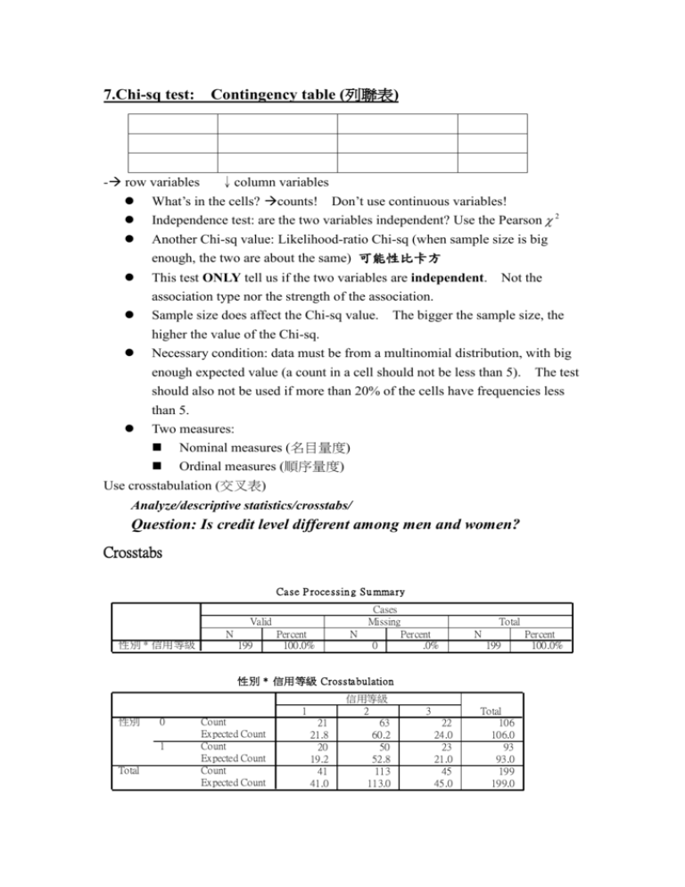
7.Chi-sq test: Contingency table (列聯表)
- row variables
↓column variables


What’s in the cells? counts! Don’t use continuous variables!
Independence test: are the two variables independent? Use the Pearson  2

Another Chi-sq value: Likelihood-ratio Chi-sq (when sample size is big
enough, the two are about the same) 可能性比卡方

This test ONLY tell us if the two variables are independent. Not the
association type nor the strength of the association.
Sample size does affect the Chi-sq value. The bigger the sample size, the
higher the value of the Chi-sq.
Necessary condition: data must be from a multinomial distribution, with big
enough expected value (a count in a cell should not be less than 5). The test
should also not be used if more than 20% of the cells have frequencies less
than 5.
Two measures:
 Nominal measures (名目量度)



 Ordinal measures (順序量度)
Use crosstabulation (交叉表)
Analyze/descriptive statistics/crosstabs/
Question: Is credit level different among men and women?
Crosstabs
Ca se P roce ssin g Su mma ry
Valid
N
性別 * 信用等級
199
Percent
100.0%
N
Cases
Missing
Percent
0
.0%
Total
N
199
性別 * 信用等級 Crossta bulation
1
性別
0
1
Total
Count
Expected Count
Count
Expected Count
Count
Expected Count
21
21.8
20
19.2
41
41.0
信用等級
2
63
60.2
50
52.8
113
113.0
3
22
24.0
23
21.0
45
45.0
Total
106
106.0
93
93.0
199
199.0
Percent
100.0%
Ch i-Sq uare Te sts
Asymp. Sig.
Value
df
(2-sided)
Pearson Chi-Square
.696a
2
.706
Likelihood Ratio
.696
2
.706
Linear-by-Linear Association
.059
1
.807
N of Valid Cases
199
a. 0 cells (.0%) have expected count less than 5. The minimum
expected count is 19.16.
Symmetric Measures
Value
Nominal by Nominal
Contingency Coefficient
Approx. Sig.
.059
N of Valid Cases
.706
199
a Not assuming the null hypothesis.
b Using the asymptotic standard error assuming the null hypothesis.
If choose “surpress table”, no table will be printed.
Question: Can we separate a continuous variable to discrete ranges
and compare?
Transform/categorize variables/  4 group
Result:
性別 * NTILES of 所得 Crosstabulation
Count
NTILES of 所得
1
性別
2
3
4
Total
0
30
37
18
21
106
1
19
13
32
29
93
49
50
50
50
199
Total
Chi-Square Tests
Asymp. Sig.
Value
Pearson Chi-Square
Likelihood Ratio
Linear-by-Linear Association
N of Valid Cases
df
(2-sided)
18.419(a)
3
.000
18.908
3
.000
9.138
1
.003
199
a 0 cells (.0%) have expected count less than 5. The minimum expected count is 22.90.
Does the result make sense? NO!!!!
Ex. Grade data
1.
2.
3.
4.
Try sex distribution in different departments?
Try Sex and living areas?
Try living areas vs. departments?
Try admission type and departments?
Different?
**Try to convert the cross tables to the following inputs.
Data input:
Use Data/Weight cases/
to give replicated frequencies
Then use Analyze/Nonparametric tests/Chi-square/
1. 適合度檢定 (test of goodness of fit) to see if the observed frequencies is as
expected
ex. 280 kids were tested for attractiveness of colors
color A
COUNT
52
B
C
D
E
F
G
48
44
31
29
30
46
Use Weight cases to assign the counts to Freq. var.
色紙
Observed N
Expected N
Residual
紅
52
40.0
12.0
橙
48
40.0
8.0
黃
44
40.0
4.0
綠
31
40.0
-9.0
藍
29
40.0
-11.0
靛
30
40.0
-10.0
紫
46
40.0
6.0
Total
280
Test Statistics
色紙
Chi-Square(a)
df
Asymp. Sig.
14.050
6
.029
a 0 cells (.0%) have expected frequencies less than 5. The minimum expected cell frequency is 40.0.
Reject Null.
The attractiveness is different.
2. Test of homogeneity proportions – to see if the responses from several
populations are different (usually an (IXJ) contingency table)
Ex. The three grades of high schools were tested for whether they wore
glasses
1st
2nd
3rd
Yes
27
34
28
No
15
12
9
Level
Grade
Freq
1
1
1
27
2
2
1
15
3
1
2
34
4
2
2
12
5
1
3
28
6
2
3
9
Data input



Weight cases  freq
Analyze/descriptive/crosstabs
Choose Chi-sq value
 row: yes, no; column: grade
有無經驗 * 年級 Crosstabulation
Count
年級
國一
國二
國三
Total
有無經
有
27
34
28
89
驗
無
15
12
9
36
42
46
37
125
Total
Chi-Square Tests
Asymp. Sig.
Value
Pearson Chi-Square
df
(2-sided)
1.506(a)
2
.471
Likelihood Ratio
1.481
2
.477
Linear-by-Linear Association
1.277
1
.259
N of Valid Cases
125
a 0 cells (.0%) have expected count less than 5. The minimum expected count is 10.66.
Can’t reject Null: No difference.
3. test of independence (or test of association) – to see if several independent
variables are related
Ex. Is education related to brand loyalty?
education
brand
loyalty
low
medium
high
University
6
17
20
High school
15
26
24
Junior high
31
34
13
Elementary
school
42
45
10
Data input
education
loyalty
freq
1
1
1
6
2
1
2
17
3
1
3
20
4
2
1
15
5
2
2
26
6
2
3
24
7
3
1
31
8
3
2
34
9
3
3
13
10
4
1
42
11
4
2
45
12
4
3
10



row: education; column: loyalty
weight cases: freq
crosstabs:
教育程度 * 社經地位 Crosst abulation
Count
低
教育
程度
Total
大學
高中
國中
國小
6
15
31
42
94
社經地位
中
17
26
34
45
122
高
Total
20
24
13
10
67
43
65
78
97
283
Ch i-Sq uare Te sts
Asymp. Sig.
Value
df
(2-sided)
Pearson Chi-Square
34.533a
6
.000
Likelihood Ratio
35.172
6
.000
Linear-by-Linear Association
30.237
1
.000
N of Valid Cases
283
a. 0 cells (.0%) have expected count less than 5. The minimum
expected count is 10.18.
Reject Null: education is related to brand loyalty.
How are they related?
Directional Measures
Value
Nominal by Nominal
Lambda
Symmetric
教育程度
Dependent
社經地位
Dependent
Goodman and
教育程度
Kruskal tau
Dependent
社經地位
Dependent
Uncertainty
Symmetric
Coefficient
教育程度
Dependent
社經地位
Dependent
Asymp. Std.
Approx.
Error(a)
T(b)
.049
.023
2.032
.042
.075
.030
2.426
.015
.019
.037
.493
.622
.039
.012
.000(c)
.051
.016
.000(c)
.051
.017
3.097
.000(d)
.046
.015
3.097
.000(d)
.058
.019
3.097
.000(d)
a Not assuming the null hypothesis.
b Using the asymptotic standard error assuming the null hypothesis.
c Based on chi-square approximation
d Likelihood ratio chi-square probability.
Symmetric Measures
Value
Approx. Sig.
Approx. Sig.
Phi
.349
.000
Cramer's V
.247
.000
Contingency
.330
Coefficient
N of Valid Cases
.000
283
a Not assuming the null hypothesis.
b Using the asymptotic standard error assuming the null hypothesis.



Note: Phi is only for 2X2 variables
Note: Contingency coeff: 2X2 or more
Note: Cramer’s V: when I is not equal to J
4. test of significance of change: to see if there is any before-and-after changes
Ex. Do you like this class:
after
before
yes
no
Yes
9
28
no
24
19
Data input
1
1
2
2
1
2
1
2



28
9
19
24
weight cases: freq.
Analyze/nonparametric tests/2 related samples/
Since we have a 2X2, choose McNemar test
學期初 & 學期末
學期末
學期初
1
2
1
28
9
2
19
24
Test Statistics(b)
學期初 &
學期末
N
Chi-Square(a)
Asymp. Sig.
a Continuity Corrected
80
2.893
.089
b McNemar Test
Fail to reject Null: Their attitude does not change.
If your data are binary, use the McNemar test. This test is typically used in a repeated
measures situation, in which each subject's response is elicited twice, once before
and once after a specified event occurs. The McNemar test determines whether the
initial response rate (before the event) equals the final response rate (after the event).
This test is useful for detecting changes in responses due to experimental
intervention in before-and-after designs.
If your data are categorical, use the marginal homogeneity test. This is an extension of the
McNemar test from binary response to multinomial response. It tests for changes in
response using the chi-square distribution and is useful for detecting response
changes due to experimental intervention in before-and-after designs. The marginal
homogeneity test is available only if you have installed Exact Tests.