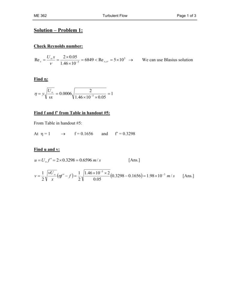
ME 362
Turbulent Flow
Page 1 of 3
Solution – Problem 1:
Check Reynolds number:
Re x 
U x


2  0.05
 6849  Re x,cr  5  10 5 
5
1.46  10
We can use Blasius solution
Find :
y
U
2
 0.0006
1
x
1.46  10 5  0.05
Find f and f’ from Table in handout #5:
From Table in handout #5:
At  = 1

f = 0.1656
and
f’ = 0.3298
Find u and v:
u  U  f   2  0.3298  0.6596 m / s
v
[Ans.]
5
1 U 
f   f   1 1.46  10  2 0.3298  0.1656  1.98  10 3 m / s
2
x
2
0.05
[Ans.]
ME 362
Turbulent Flow
Page 2 of 3
Solution – Problem 2:
Determine if flow is laminar or turbulent:
Since we don’t know if the flow at x = 2.0 m is laminar or turbulent, we will begin with
laminar flow analysis. If this doesn’t work, we can switch to turbulent analysis.
Let us assumed the flow is laminar first:
3
2
 w  0.332U 

x
3
w
x
0.332 

U 2 

 
x 3

U    w

0
.
332




 2.1
2
U   
5
 0.332 1.2  1.8  10
2
155  2
 20.67  10 6  Re x,cr  5  10 5
5
1.5  10
Re x 
U x

laminar flow assumption is wrong


2
3
  155 m / s


1
  6U 13  7

 w  0.0135
x


13
7

w
1
 x 7



0.0135   6 

U

1 13




w
x 7



U 
 0.0135   6  




2.1 
2

U  


 0.0135  1.8  10 5  1.2 6 

7
34  2
 4.53  10 6  Re x,cr  5  10 5
5
1.5  10
Re x 
U x

turbulent flow assumption is correct

U   34 m / s


[Ans.]
1
7




7
13
 34 m / s
ME 362
Turbulent Flow
Page 3 of 3
Find  at x = 2 m:

x

0.16
Re

1
7
x
 
0.16 x
Re
1
7
x

0.16  2
(4.53  10 6 )
1
7
 3.58  10  2 m
[Ans.]
Find u at y = 4 cm:
y = 4 cm
BL
 = 3.58 cm
x=2m
At y = 4 cm >  = 3.58 cm

we reach the free stream region

u  U   34 m / s
1
[Ans.]
u
 y 7
Note: We can use 1/7th power law (i.e.,
   ) if the y location is inside the
U  
boundary layer.