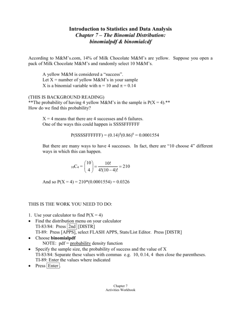
Introduction to Statistics and Data Analysis
Chapter 7 – The Binomial Distribution:
binomialpdf & binomialcdf
According to M&M’s.com, 14% of Milk Chocolate M&M’s are yellow. Suppose you open a
pack of Milk Chocolate M&M’s and randomly select 10 M&M’s.
A yellow M&M is considered a “success”.
Let X = number of yellow M&M’s in your sample
X is a binomial variable with n = 10 and  = 0.14
(THIS IS BACKGROUND READING)
**The probability of having 4 yellow M&M’s in the sample is P(X = 4).**
How do we find this probability?
X = 4 means that there are 4 successes and 6 failures.
One of the ways this could happen is SSSSFFFFFF
P(SSSSFFFFFF) = (0.14)4(0.86)6 = 0.0001554
But there are many ways to have 4 successes. In fact, there are “10 choose 4” different
ways in which this can happen.
10C4
10 
10!
=  
 210
 4  4!(10  4)!
And so P(X = 4) = 210*(0.0001554) = 0.0326
THIS IS THE WORK YOU NEED TO DO:
1. Use your calculator to find P(X = 4)
 Find the distribution menu on your calculator
TI-83/84: Press 2nd [DISTR]
TI-89: Press [APPS], select FLASH APPS, Stats/List Editor. Press [DISTR]
 Choose binomialpdf
NOTE: pdf = probability density function
 Specify the sample size, the probability of success and the value of X
TI-83/84: Separate these values with commas e.g. 10, 0.14, 4 then close the parentheses.
TI-89: Enter the values where indicated
 Press Enter .
Chapter 7
Activities Workbook
How about probability of “at most” 4 yellow M&M’s?
P(X  4) = ???
You could find the individual probabilities for X = 0, 1, 2, 3, 4 and add them up.
OR
2. Use your calculator to find P(X  4)
 Get to the distribution menu.
 Choose binomialcdf
NOTE: cdf = cumulative distribution function
 Specify the sample size, the probability of success and the value of X
TI-83/84: Separate these values with commas e.g. 10, 0.14, 4 then close the parentheses.
TI-89: Enter the values where indicated
 Press Enter .
P(X  4) =
3.





Find the probabilities for each possible X value.
Put all the possible values of X (0, …, 10) into a column (e.g. L1 or list1) .
Put the cursor onto the name of the next column, (e.g. onto L2 or list2)
Get to the distribution menu
Choose the binomial pdf.
Specify the sample size, the probability of success and the column of X values
TI-83/84: 10, 0.14, L1)
TI-89: Enter the values where indicated, using the column of X values
The lists in your calculator tell you the chance that your sample will have zero “successes”, one
“success”, two “successes”, etc. (remember, “success” = yellow).
A sample with
yellow M&M’s is most likely to occur.
4. Make a scatterplot– your Xlist is the possible X values and your Ylist is the probabilities.
Because the probabilities on the Y-axis are basically relative frequency, we could replace the
points on the graph with bars from the X-axis up to each point and make a histogram. (This
requires several steps. We won’t worry about it.)
5. Describe the graph as follows:
Mode (value of X with the highest bar):
Range of likely values (values of X with bars above zero):
Shape of the graph (describe as you would a histogram):
Chapter 7
Activities Workbook
Solution To Binomial Distribution
Let X = number of yellow M&M’s in your sample
X is a binomial variable with n = 10 and  = 0.14
1. P(X = 4) = binomialpdf(10, 0.14, 4) = 0.0326
2. P(X  4) = binomialcdf(10, 0.14, 4) = 0.9927
3. A sample with 1 yellow M&M is most likely to occur.
L1
L2
0
0.2213015789
1
0.3602583842
**highest prob
2
0.2639102117
3
0.1145656733
4
0.0326378953
5
0.0063757749
6
0.0008649307
7
0.0000804587
8
0.0000049117
9
0.0000001777
10
0.0000000029
4. and 5. Mode: X = 1
Range of likely values of X: 0 to 5
The graph is unimodal and skewed to the right.
Scatterplot of P(X = x) vs x
0.4
P(X = x)
0.3
0.2
0.1
0.0
0
2
4
6
x
Chapter 7
Activities Workbook
8
10
Introduction to Statistics and Data Analysis
Chapter 7 – The Normal Distribution:
normalcdf & invNorm
HEY! Read this section first.
Find the probability distributions menu on your calculator:
TI-83/84
2nd [DISTR]
TI-89
Go to the Stat/List Editor, then press DISTR (F5)
There are three choices involving the normal distribution
normalpdf(x, , )
Gives the height of the curve at x. NOT a probability.
NOTE: NEVER use normalpdf
normalcdf(lowerbound, upperbound, , )
Computes the probability P(lowerbound < X < upperbound)
TI-83/84: invNorm(p, , )
TI-89: Inverse Normal (NOTE: Area is p)
Computes the 100pth percentile of X
(e.g., using 0.25 for p will give the 25th percentile of X)
Now give it a try! Suppose X ~ N(25, 8).
1. Find P(17 < X < 23).
2. Find P(X < 10).
HINT: The lower bound for this probability is -. The TI-83/84 don’t recognize -, so use a
very negative number instead, e.g. –10000.
3. Find P(X > 32).
HINT: The upper bound is . The TI-83/84 don’t recognize , so use a very positive number
instead, e.g. 10000.
4. Find the 10th percentile of X.
Chapter 7
Activities Workbook
Ready for more?
Let X ~ N(0,1).
1. Find P(X < 0)
2. Find P(-1 < X < 1)
3. Find P(-2 < X < 2)
4. Find P(-3 < X < 3)
Are these probabilities familiar? They are used in the _____________ Rule.
One more time!
Suppose IQ scores are normally distributed with a mean of 100 and a standard deviation of 15.
1. What is the probability that a person has an IQ score greater than 120?
2. What is the probability that a person has an IQ score between 110 and 130?
3. What is the 90th percentile of IQ scores?
4. 2% of IQ scores are above __________. (HINT: What percentile is this?)
Chapter 7
Activities Workbook
Solution To Normal Distribution
Part I
1. normalcdf(17, 23, 25, 8) = 0.2426
2. normalcdf(-10000, 10. 25. 8) = 0.0304
3. normalcdf(32, 10000, 25, 8) = 0.1908
4. invNorm(0.10, 25, 8) = 14.75
Part II.
1. normalcdf(-10000,0,0,1) = 0.5
2. normalcdf(-1,1,0,1) = 0.6827
3. normalcdf(-2,2,0,1) = 0.9545
4. normalcdf(-3,3,0,1) = 0.9973
These probabilities are used in the EMPIRICAL Rule.
Part III.
1. normalcdf(120,10000,100,15) = 0.0912
2. normalcdf(110,130, 100, 15) = 0.2297
3. invNorm(0.90, 100, 15) = 119.22
4. invNorm(0.98, 100, 15) = 130.81
Chapter 7
Activities Workbook
Introduction to Statistics and Data Analysis
Chapter 7 – Assessing Normality
1. Based on the normal probability plot below, does it appear that a normal probability model is
appropriate for this data? EXPLAIN.
Normal Probability Plot
99
95
90
80
Percent
70
60
50
40
30
20
10
5
1
0
20
40
60
80
100
120
140
160
2. The normal probability plots below have “confidence bands”. For a normal probability model
to be appropriate, almost all points should be within the confidence bands.
For each of the normal probability plots below, does it appear that a normal probability model is
appropriate for the data? EXPLAIN.
Normal Probability Plot of A
99
95
90
80
Percent
70
60
50
40
30
20
10
5
1
50
75
100
A
125
150
Normal Probability Plot of B
99
95
90
80
Percent
70
60
50
40
30
20
10
5
1
-50
-25
0
25
50
75
100
125
B
Normal Probability Plot of C
99
95
90
80
Percent
70
60
50
40
30
20
10
5
1
0
1
2
3
4
5
6
7
8
9
C
Chapter 7
Activities Workbook
3. IQ scores for a random sample of people are shown below.
72
79
87
91
99
101
103
106
111
113
116
126
A. Make a normal probability plot and draw it below.
TI-83/84: Make a STATPLOT, using the last graph “Type”
TI-89: In the Stat/List Editor, set up the plot (choose Plots (F2) and select Normal Prob
Plot), then graph the plot (choose Plots (F2) and select Plot Setup)
B. Based on this sample, is a normal probability model appropriate for IQ scores? EXPLAIN.
Chapter 7
Activities Workbook
Solution to Assessing Normality
1. NO, a normal probability model is not appropriate because the normal probability plot is not a
straight line (it is a curve!).
2. A. YES, a normal probability model is appropriate because the normal probability plot is a
straight line (almost all points within the confidence bands).
B. NO, a normal probability model is not appropriate because the normal probability plot is
not a straight line (many points outside the confidence bands).
C. YES, a normal probability model is appropriate because the normal probability plot is a
straight line (almost all points within the confidence bands). (But, since graph looks curved,
not straight, COULD BE INTERPRETED EITHER WAY)
3. A. Normal Probability Plot of the sample of IQ scores
Normal Probability Plot of IQ
99
95
90
80
Percent
70
60
50
40
30
20
10
5
1
70
80
90
100
IQ
110
120
130
B. The normal probability plot is approximately a straight line, so a normal probability model
is appropriate for IQ scores.
Chapter 7
Activities Workbook