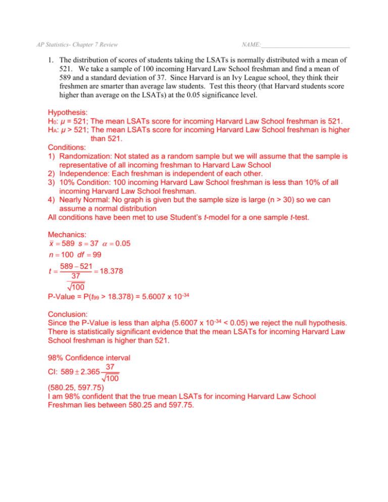
AP Statistics- Chapter 7 Review
NAME:____________________________
1. The distribution of scores of students taking the LSATs is normally distributed with a mean of
521. We take a sample of 100 incoming Harvard Law School freshman and find a mean of
589 and a standard deviation of 37. Since Harvard is an Ivy League school, they think their
freshmen are smarter than average law students. Test this theory (that Harvard students score
higher than average on the LSATs) at the 0.05 significance level.
Hypothesis:
H0: µ = 521; The mean LSATs score for incoming Harvard Law School freshman is 521.
HA: µ > 521; The mean LSATs score for incoming Harvard Law School freshman is higher
than 521.
Conditions:
1) Randomization: Not stated as a random sample but we will assume that the sample is
representative of all incoming freshman to Harvard Law School
2) Independence: Each freshman is independent of each other.
3) 10% Condition: 100 incoming Harvard Law School freshman is less than 10% of all
incoming Harvard Law School freshman.
4) Nearly Normal: No graph is given but the sample size is large (n > 30) so we can
assume a normal distribution
All conditions have been met to use Student’s t-model for a one sample t-test.
Mechanics:
x  589 s  37   0.05
n  100 df  99
589  521
t
 18.378
37
100
P-Value = P(t99 > 18.378) = 5.6007 x 10-34
Conclusion:
Since the P-Value is less than alpha (5.6007 x 10-34 < 0.05) we reject the null hypothesis.
There is statistically significant evidence that the mean LSATs for incoming Harvard Law
School freshman is higher than 521.
98% Confidence interval
37
CI: 589  2.365
100
(580.25, 597.75)
I am 98% confident that the true mean LSATs for incoming Harvard Law School
Freshman lies between 580.25 and 597.75.
2. A teacher wants to test the effectiveness of a new textbook. She believes that this new textbook
is easier to read, and that students should have better grades on their tests than they have in the
past. She collected the following test scores from SRSs from all of last year’s and this year’s
classes. Assume normal populations for both years, and assume these are SRSs from the entire
population of students who use this text book. Test her theory at the 0.01 significance level.
Old book
85 84
75 82
74 64
91
84
58
75
89
95
65
62
50
New book
94 62 86
96 88 88
94 84 86
89
79
78
80
75
64
Hypothesis:
H0: µO – µN = 0; There is no difference in the mean test scores from last year using the old
book and this year using the new book.
HA: µO – µN < 0; The mean test scores from last year are lower than the mean scores from
this year.
Conditions:
1) Randomization: Stated as random samples
2) Independence: The two classes would be independent of each
other
3) Nearly Normal: Histograms are unimodal and approximately
symmetric
All conditions have been met to use Student’s t-model for a two
sample t-test.
Mechanics:
nO  15 xO  75.53 sO  13.27   0.01
nN  15 xN  82.87 sN  10.11
df  26.2
75.53  82.87
t
 1.703
13.272 10.112

15
15
P-Value = P(t26.2 < -1.703) = 0.0502
Conclusion:
Since the P-Value is greater than alpha (0.0502 > 0.01) we fail to reject the null
hypothesis. There is not enough evidence to state that the mean scores from last year
were less than this year. There is not enough evidence to state that the students perform
better with the new textbook.
13.272 10.112

 ( 16.18,1.517)
15
15
I am 95% confident that the mean scores of students that used the old book is between
16.18 points lower and 1.517 points higher than for students that used the new book.
CI:  75.53  82.87   2.055
3. A football coach is frustrated with his team’s lack of speed. He measures each player’s 40-yard
dash speed and then sends all of them to a speed and agility camp. He then measures their
times again after. The data is below. Is their sufficient evidence at the 0.05 significance level
to say that the camp helped the players speed?
Before
After
4.88
4.7
5.1
4.85
4.41
4.35
4.73 4.6 4.8 4.95 4.98 5.2 5.13 5.05 4.9 4.7 4.6 5.11
4.77 4.56 4.78 4.7 4.9
5
5.1 5.1 4.7 4.56 4.34 4.9
Hypothesis:
H0: µBefore – After = 0; The mean difference in time before the camp and after the camp is
zero.
HA: µBefore – After > 0; The mean difference in time before the camp and after the camp is
greater than zero. There has been a reduction in the time of a player’s 40yard dash.
Conditions:
1) Randomization: Not stated as a random sample but we will assume that the sample is
representative of all football players
2) Independence: Each player is independent of each other.
3) Nearly Normal: The normal probability plot show an approximately linear pattern
All conditions have been met to use Student’s t-model for a one sample t-test.
Mechanics:
xd  0.122 sd  0.108   0.05
n  15 df  14
0.122  0
t
 4.387
0.108
15
P-Value = P(t14 > 4.387) = 3.103 x 10-4
Conclusion:
Since the P-Value is less than alpha (3.103 x 10-4 < 0.05) we reject the null hypothesis.
There is statistically significant evidence that the mean difference in times from before the
camp to after the camp has decreased. The camp has helped the player’s speed.
CI: 0.122  1.761
0.108
 (0.073,0.171)
15
I am 90% confident that the mean difference in times from before the camp to after the
camp lies between 0.073 to 0.171 seconds.
4. Poisoning by DDT causes tremors and convulsions and slows recovery times of muscles. In a
study of DDT poisoning, researchers fed several lab rats a measured amount of DDT. They
then made measurements of the rats’ refractory period (the time needed for a nerve to recover
after a stimulus). They know that the mean time for unpoisoned rats is 1.3 milliseconds and
that these times vary normally. In their sample they find the following times:
1.61 1.9
1.53 1.4
1.33 1.81 1.3
1.25 1.65
Test the hypotheses that DDT poisoning should slow nerve recovery and thus increase the
refractory times.
Hypothesis:
H0: µ = 1.3; The mean refractory period is 1.3 milliseconds
HA: µ > 1.3; The mean refractory period is more than 1.3 milliseconds
Conditions:
1) Randomization: Not stated as a random sample but we will assume that the sample is
representative of all rats
2) Independence: Each rat is independent of each other.
3) Nearly Normal: The normal probability plot shows an approximate linear pattern
All conditions have been met to use Student’s t-model for a one sample t-test.
Mechanics:
x  1.531 s  0.230   0.05
n  9 df  8
1.531  1.31
t
 3.011
0.230
9
P-Value = P(t8 > 3.011) = 0.0084
Conclusion:
Since the P-Value is less than alpha (0.0084 < 0.05) we reject the null hypothesis. There
is statistically significant evidence that the mean refractory period for mice poisoned with
DDT is lower than 1.3 milliseconds.
5. Chapin Social Insight Test is a psychological test designed to measure how accurately a person
appraises other people. The possible scores on the test range from 0 to 41. During the
development of the test, it was given to several groups of people. Here are the results for male
and female college students at a liberal arts college:
Male
Female
N
133
162
x
25.34
24.94
s
5.05
5.10
Does the data support the contention that female and male students differ in average social
insight?
Hypothesis:
H0: µM – µF = 0; There is no difference in the mean score on the Chapin Social Insight
Test for males compared to females.
HA: µM – µF ≠ 0; There is a difference in the mean score on the Chapin Social Insight Test
for males compared to females.
Conditions:
1) Randomization: Not stated as random so we will assume that each sample is
representative of the two populations
2) Independence: Males and females would be independent of each other
3) Nearly Normal: No graphs were given but the sample sizes are both large (n > 30) so
we assume normal distributions.
All conditions have been met to use Student’s t-model for a two sample t-test.
Mechanics:
nM  133 xM  25.34 sM  5.05   0.05
nF  162 xF  24.94 sF  5.10
df  282.95
25.34  24.94
t
 0.674
5.052 5.102

133
162
P-Value = 2P(t282.95 > 0.674) = 0.2505
Conclusion:
Since the P-Value is greater than alpha (0.2502 > 0.05) we fail to reject the null
hypothesis. There is not enough evidence to state that there is a difference in the mean
scores of males compared to females on the Chapin Social Insight Test.
6.
Hypothesis:
H0: µregular-premium = 0; The mean difference of mpg between regular gasoline and premium
gasoline is zero.
HA: µregular-premium < 0; The mean difference of mpg between regular gasoline and premium
gasoline is less than zero.
Conditions:
1) Paired data: Data is from individual cars using both regular and premium gasoline.
2) Randomization: Each car is randomly assigned to a treatment
3) Independence: Each car’s mpg would be independent of each other
4) Nearly Normal: The normal probability plot of the differences is
approximately linear with no large outliers.
All conditions have been met to use Student’s t-model for a matched pairs t-test.
Mechanics:
xd  2 sd  1.414   0.05
n  10 df  9
2  0
t
 4.472
1.414
10
P-Value = P(t9 < -4.472) = 7.749 x 10-4
Conclusion:
Since the P-Value is less than alpha (7.749 x 10-4 < 0.05) I would reject the null
hypothesis. There is statistically significant evidence that mean difference of mpg between
regular and premium gasoline is less than zero. It appears that cars get better mpg using
premium gasoline.