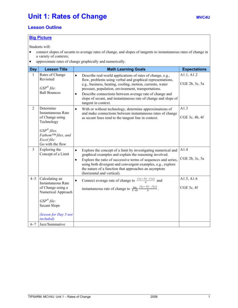
Unit 1: Rates of Change
MVC4U
Lesson Outline
Big Picture
Students will:
• connect slopes of secants to average rates of change, and slopes of tangents to instantaneous rates of change in
a variety of contexts;
• approximate rates of change graphically and numerically.
Day
Lesson Title
1 Rates of Change
Revisited
GSP® file:
Ball Bounces
2
3
Determine
Instantaneous Rate
of Change using
Technology
GSP® files,
Fathom™ files, and
Excel file:
Go with the flow
Exploring the
Concept of a Limit
Math Learning Goals
•
•
•
•
•
4–5 Calculating an
•
Instantaneous Rate
of Change using a
Numerical Approach
Expectations
A1.1, A1.2
Describe real-world applications of rates of change, e.g.,
flow, problems using verbal and graphical representations,
CGE 2b, 3c, 5a
e.g., business, heating, cooling, motion, currents, water
pressure, population, environment, transportations.
Describe connections between average rate of change and
slope of secant, and instantaneous rate of change and slope of
tangent in context.
A1.3
With or without technology, determine approximations of
and make connections between instantaneous rates of change
CGE 3c, 4b, 4f
as secant lines tend to the tangent line in context.
Explore the concept of a limit by investigating numerical and A1.4
graphical examples and explain the reasoning involved.
Explore the ratio of successive terms of sequences and series, CGE 2b, 3c, 5a
using both divergent and convergent examples, e.g., explore
the nature of a function that approaches an asymptote
(horizontal and vertical).
f (a + h) − f (a)
A1.5, A1.6
Connect average rate of change to
and
h
instantaneous rate of change to
lim f ( a + h ) − f ( a )
h →0
h
.
CGE 3c, 4f
GSP® file:
Secant Slope
(lesson for Day 5 not
included)
6–7 Jazz/Summative
TIPS4RM: MCV4U: Unit 1 – Rates of Change
2008
1
Unit 1: Day 1: Revisiting Rates of Change
MVC4U
Math Learning Goals
Describe real-world applications of rates of change using verbal and graphical
representations, e.g., business, heating, cooling, motion, currents, water pressure,
population, environment, transportation.
• Describe connections between average rate of change and instantaneous rate of
change in context.
•
Materials
• chart paper and
markers
• computer and
data projector
• BLMs 1.1.1–1.1.5
75 min
Assessment
Opportunities
Minds On… Groups Æ Graffiti
Post seven pieces of chart paper each containing a term students encountered in
MHF4U. Give each group a different coloured marker.
In heterogeneous groups of three or four students have 30 seconds to write
anything they know about the term using numbers, symbols, and/or words.
Groups move through all seven charts.
Whole Class Æ Discussion
Using the four scenarios provided on BLM 1.1.1, review connections between
rates of change and the slopes of secants and tangents.
Guiding questions:
• Describe the rate of change of the walleye population over the 25 year period.
• Would you expect half of the water to drain in half the time? Justify.
• What is the rocket’s instantaneous rate of change at four seconds? Describe
what the rocket is doing at this point of time.
• Although the Ferris wheel is turning at a constant rate, the rate of change of
height is not constant. Explain why.
Word Wall
• dependent variable
• independent
variable
• finite differences
• slope of secant line
• slope of tangent
line
• average rate of
change
• instantaneous rate
of change
See pp. 66–68
Think Literacy:
Cross-Curricular
Approaches,
Grades 7–12 for
more information on
Graffiti.
®
Action!
Pairs Æ Investigation
Curriculum Expectation Observation/Mental Note: Observe to identify
students’ ability to make connections between the average rate of change and
slope of secant and instantaneous rate of change and slope of tangent.
Students complete the investigation on average and instantaneous rates of change
from BLM 1.1.2.
Mathematical Process Focus: Connecting
GSP sketch Ball
Bounces.gsp can be
used to demonstrate.
Make use of an
interactive
whiteboard, if
available.
Consider using a
computer lab with
®
GSP to complete
the investigation on
BLM 1.1.2.
Consolidate Whole Group Æ Discussion
Debrief
Share findings with the class. Address any misunderstandings.
Guiding Questions:
• Describe how to select points on a curve so that the slope secant better
represents the instantaneous rate of change at any point in the interval.
• How would you change the intervals around each bounce to provide better
information about the average and instantaneous rates of change of the ball?
Pairs Æ Pair/Share: Frayer Model
A coaches B in completing a Frayer model for average rate of change. B coaches
A in completing Frayer model for instantaneous rate of change (BLM 1.1.4).
Application
See pp. 162–165 of
Think Literacy:
Cross-Curricular
Approaches,
Grades 7–12 for
more information on
Frayer Models.
Home Activity or Further Classroom Consolidation
Gather examples of rates of change from your life using Worksheet 1.1.5.
TIPS4RM: MCV4U: Unit 1 – Rates of Change
2008
2
1.1.1: Revisiting Rates of Change
1.
25-year Walleye Population
Year
0
1
2
3
4
5
6
7
8
9
10
11
12
13
14
15
16
17
18
19
20
21
22
23
24
25
Walleye Population
3000
3400
3720
3976
4181
4345
4476
4581
4665
4732
4786
4829
4863
4890
4912
4930
4944
4955
4964
4971
4977
4982
4986
4989
4991
4993
A Fish Story
A pond was stocked with a type of fish called "walleye.”
The table on the left gives the population of walleye in the
pond for the 25 years following the stocking of the pond.
2.
Down the Drain
The plug is pulled in a small hot tub. The table on
the right gives the volume of water in the tub from
the moment the plug is pulled, until it is empty.
Source:
http://www.clipsahoy.com/webgraphics/as0963.htm
TIPS4RM: MCV4U: Unit 1 – Rates of Change
Draining Water
from a Hot Tub
Time (s)
Volume (L)
0
10
20
30
40
50
60
70
80
90
100
110
120
2008
1600
1344
1111
900
711
544
400
278
178
100
44
11
0
3
1.1.1: Revisiting Rates of Change (continued)
3.
Blast Off
A rocket is launched.
The graph shows its
height above the
ground from time of
launching to return to
earth.
4.
TIPS4RM: MCV4U: Unit 1 – Rates of Change
2008
4
1.1.2: That’s the Way the Ball Bounces!
Kevin dropped a ball and collected the height (m) at various times (s). A graph of the data he
collected is provided.
Part A: Average Rate of Change
Kevin wants to look at rate of change of the height at various times. He hopes to determine how
quickly the height was changing at various times. Kevin first looks at the average rate of change
for specific time intervals. Complete the table with the information in the graph.
Interval
Average
Rate of Change
Coordinates of End Points
AB
BC
CD
DE
EF
FG
GH
What do the values for average rate of change tell you about the path of the ball and the speed
of the ball?
TIPS4RM: MCV4U: Unit 1 – Rates of Change
2008
5
1.1.2: That’s The Way the Ball Bounces! (continued)
Part B: Instantaneous Rate of Change
Next, Kevin wants to find a point in each interval whose tangent has the same instantaneous
rate of change as each secant.
Sketch a curve of best fit for this data in one colour and draw the secants for the intervals in
another colour.
For each time interval, locate the point on the graph between the endpoints whose tangent
appears to have the same rate of change as the average rate of change for that interval.
1. On the interval AB the average rate of change is ___________. The point whose tangent
matches this rate of change is (________, ________). Draw the instantaneous rate of
change at this point, if possible.
2. On the interval BC, the average rate of change is ___________. The point that most closely
matches this rate of change is (________, ________).
3. On the interval CD, the average rate of change is ___________. The point that most closely
matches this rate of change is (________, ________). Draw the tangent at this point, if
possible.
4. On the interval EF, the average rate of change is ___________. The point that most closely
matches this rate of change is (________, ________). Draw the tangent at this point, if
possible.
TIPS4RM: MCV4U: Unit 1 – Rates of Change
2008
6
1.2.2: That’s The Way the Ball Bounces! (continued)
5. On the interval GH, the average rate of change is ____________. The point that most
closely matches this rate of change is (______, ______).
Kevin notices some problems for some of the intervals.
a) For which intervals is it difficult to find a matching point?
b) Why is if difficult to find instantaneous rate of change for these intervals?
c) What was happening to the motion of the ball in these intervals?
TIPS4RM: MCV4U: Unit 1 – Rates of Change
2008
7
1.1.3: That’s The Way the Ball Bounces! (Teacher)
The following provides the coordinates of all the data points gathered by the ball bounce
experiment.
Time
(s)
0.00
0.03
0.07
0.10
0.13
0.17
0.20
0.23
0.26
0.30
0.33
0.36
0.40
0.43
0.46
0.50
0.53
0.56
0.59
0.63
0.66
0.69
0.73
0.76
0.79
0.83
0.86
0.89
0.92
0.96
0.99
1.02
1.06
Height
(cm)
212
182
147
103
55
0
40
80
114
141
161
177
182
182
178
164
146
118
87
49
2
30
63
89
108
120
129
126
121
105
86
63
27
TIPS4RM: MCV4U: Unit 1 – Rates of Change
2008
8
1.1.4: Frayer Model
Name: ______________________________________Date: _____________________
Definition
Examples
TIPS4RM: MCV4U: Unit 1 – Rates of Change
Characteristics
Average Rate
of Change
Non-Examples
2008
9
1.1.4: Frayer Model (continued)
Definition
Examples
TIPS4RM: MCV4U: Unit 1 – Rates of Change
Characteristics
Instantaneous
Rate of
Change
Non-Examples
2008
10
1.1.4: Frayer Model Solutions (Teacher)
Definition
Characteristics
Average Rate of Change is the measure of the rate of change for
a continuous function over a time interval.
•
•
•
•
The rate can be represented as the slope of a secant line
between the end points of the interval
The slope of the secant line is equivalent to the average
rate of change
Cannot be determined over intervals for functions that have
non-continuous intervals such as cusps and vertical
asymptotes
The sign of the slope indicates whether a function is
increasing or decreasing
Average Rate
of Change
Examples
Average speed of a car for a trip
distance travelled
Speed =
elapsed time
•
•
•
Non-Examples
Average height
Average class mark
Average income of families
Average rate of bacteria growth
Slope of Secant =
f ( a + h) − f ( a )
h
TIPS4RM: MCV4U: Unit 1 – Rates of Change
2008
11
1.1.4: Frayer Model Solutions (Teacher)
Definition
Characteristics
Instantaneous Rate of Change is the measure of the rate of
change for a continuous function at point on the function.
•
•
•
•
Examples
Instantaneous
Rate of
Change
Real-time readout of speed of a car.
Real-time readout of a geiger counter measuring radioactivity
Slope of Tangent to a curve
TIPS4RM: MCV4U: Unit 1 – Rates of Change
The rate can be represented as the slope of the tangent
line to a curve at a particular point
The slope of the tangent line is equivalent to the
instantaneous rate of change
Cannot be determined when there is a drastic change in
the motion of an object such as at the point an object
bounces
Cannot be determined for functions that are not continuous
or have vertical asymptotes
•
•
Non-Examples
Average rate of change of a function
Gauges that do not measure rates such as: odometer in a
car, altimeter in an aircraft, …
2008
12
1.1.5: Bringing It All Together
Describe an example in your life that matches each of the following situations. Explain why you
believe each situation models the requirements stated.
Use any of the examples or situations different from those discussed in class!
1. Positive average rate of change all of the time.
2. Positive average rate of change sometimes and a negative average rate of change
sometimes.
3. Instantaneous rate of change equal to zero at least once.
4. Instantaneous rate of change which cannot be calculated at least once.
TIPS4RM: MCV4U: Unit 1 – Rates of Change
2008
13
GSP® File: Ball Bounces
TIPS4RM: MCV4U: Unit 1 – Rates of Change
2008
14
Unit 1: Day 2: Go with the Flow
MVC4U
Math Learning Goals
Make connections with or without graphing technology between an approximate
value of the instantaneous rate of change at a given point on the graph of a smooth
function and average rates of change over intervals containing the point.
• Use the slopes of a series of secants through a given point on a smooth curve to
approximate the slope of the tangent at the point.
•
Materials
• BLMs 1.2.1–1.2.6
• plastic bottles
• 1-2L graduated
cylinders or
measuring cups
• water
• stop watch
75 min
Assessment
Opportunities
Minds On… Pairs Æ Think/Pair/Share
Use the context of water flowing out of a water reservoir tank and BLMs 1.2.1
and 1.2.2 to activate prior knowledge about average and instantaneous rate of
change and to determine what students know about rate of change.
Go with the flow.ftm
Go with the flow
exemplar.ftm
Go with the flow
exemplar2.ftm
Go with the
flow.gsp
Go with the flow
exemplar.gsp
Go with the flow.xls
Action!
Small Groups Æ Investigation
Curriculum Expectation/Observation/Mental Note: Observe to identify
students’ ability to make connections between the average rate of change over an
interval containing a point and the instantaneous rate of change at a given point.
Students work in groups of three or four using BLM 1.2.3 to understand the
instantaneous rate of change of the volume of water as it flows out of a container
with respect to time and to recognize this to be the instantaneous rate of flow.
Students approximate the instantaneous rate of water flowing from a plastic
drink container into a measuring cup or graduated cylinder, using a series of
secants to the graph showing the relationship between the volume of water
flowing out of the plastic drink container and time.
Differentiating Instruction: The investigation can be changed to “height versus
time” by placing a measured tape on the straight side of the container and
adjusting the BLM appropriately.
Mathematical Process Focus: Connecting, Selecting Tools and Strategies.
Collect and prepare
plastic cylindrical
containers of various
sizes.
Cards (BLM 1.2.4)
are available to
provide additional
scaffolding.
BLM 1.2.5 provides
instructions for using
technology to graph
the data and find
slopes of secants.
Consolidate Whole Class Æ Discussion
Debrief
Students share results and strategies used to answer the questions in the
investigation (BLM 1.2.3). Use the points made by students to consolidate the
following:
• The difference between average and instantaneous rate of water flow.
• The connection between average rate of water flow with secants and
instantaneous rate of water flow with tangents to the graph.
• The challenge of determining the instantaneous rate of water flow.
• The use of secants (or average rates of water flow) to approximate the
instantaneous rate of water flow at a given point in time.
Concept Practice
Home Activity or Further Classroom Consolidation
Consolidate your learning (Worksheet 1.2.6).
TIPS4RM: MCV4U: Unit 1 – Rates of Change
2008
15
1.2.1: Think/Pair/Share
Context
Answer each question regarding how water will flow out of the water
reservoir shown. Assume the tank is cylindrical and the water is
draining out of the bottom of the tank.
1. Do you think the rate of flow of the water out of the reservoir tank
is constant? Explain your reasoning.
Image source:
home.att.net/~berlinerUltrasonics/bwzsagAa6.html
2. Using Worksheet 1.2.2, consider possible models for the relationship between the volume of
water flowing out of the reservoir tank and time.
a) Which model(s) would you immediately dismiss and why?
b) Which graph best models the relationship between the total water that has flowed out of
the tank and time? Justify your choice.
3. The average rate of flow is a measure of the rate of change of the volume of water that has
flowed out of the reservoir over a given time interval. Use the graph chosen above to explain
how the average rate of flow changes as the reservoir empties.
4. Describe the difference between an average rate of flow and an instantaneous rate of flow.
TIPS4RM: MCV4U: Unit 1 – Rates of Change
2008
16
1.2.2: Average and Instantaneous Rate of Change
Each graph models a relationship between the total volume (mL) of water that has flowed out of
the tank and time(s).
TIPS4RM: MCV4U: Unit 1 – Rates of Change
2008
17
1.2.3: Go with the Flow
Context: To investigate the rate that water
flows out of a cylindrical water tower.
Preparing Materials: Using a plastic drinking
container (1.5–2L) make a 3–5 mm hole above
the ridges on the bottom of the plastic drinking
container. Set up the apparatus as shown in
the diagram:
Step One: Gather volume and time data as
one litre of water flows out of the plastic
drinking container into a measuring cup or graduated cylinder. Record the time at which the
volume in the measuring cup reaches a multiple of 50mL in the chart below:
Graph the data, Volume versus Time, using graph paper or graphing
technology, e.g., graphing calculators, Excel or Fathom™.
Step Two: Construct a curve of best fit with or without technology.
Time
(s)
0
Volume
(mL)
0
50
100
Step Three: Calculate the average rate of water flow over the whole time
interval. (Card 1) What connections can you make between the average
rate of water flow over the whole time interval and the secant to the graph
at the endpoints? (Card 2)
Step Four: Repeat Step 3 choosing two different points on the curve.
What connections can you make between instantaneous flow rates at a
specific time and tangents to the graph? (Card 3)
Approximate the instantaneous rate of flow, when 750 mL of water has
been collected in the measuring cup, by using your graph and a series of
secants containing the point. (Card 4)
150
200
250
300
350
400
450
500
Step Five: Specifications for the water tower require that the rate of flow
cannot be less than half the initial instantaneous flow rate.
What is the initial instantaneous rate of flow?
Investigate whether or not the rate of flow will meet the required
specifications:
• when the container is half full.
• when the container is a quarter full.
550
600
650
700
750
800
Determine the time when the flow rate is exactly half the initial
instantaneous flow rate.
850
900
950
1000
TIPS4RM: MCV4U: Unit 1 – Rates of Change
2008
18
1.2.4: Hint Cards
Hint 1
Average Flow Rate =
Volume Collected
Time Interval
If 200mL flows out of the container in 10 seconds, the average rate that the water flows out
of the container is:
Average Flow Rate =
Volume Collected 200mL
mL
=
= 20
Time Interval
10s
s
Hint 2
A secant is a line that intersects a curve at two points. Find the slope of the secant using
the first and last points on the graph. Compare with the average flow rate.
Hint 3
A tangent is a line that makes contact with a curve at one point, without intersecting it.
Find the slope of the tangent using two points on the line. Compare with the instantaneous
flow rate.
Hint 4
To use secants to approximate the slope of a given tangent find the slopes of secants
with end points on either side of the point of tangency. To get better estimates of the
slope of the tangent, make the end points of the secant closer to the point of tangency.
TIPS4RM: MCV4U: Unit 1 – Rates of Change
2008
19
1.2.5: Go With the Flow:
Average and Instantaneous Rate of Change
Analysis of Data using Fathom™
1. Open the data collection: Go with the flow.ftm.
2. Complete Step 1 by clicking on the table and entering each time and volume measurement.
Note that because the volume collected is definitely 0 mL at time 0 s, record this data point
first. If you are missing some volume-time measurements simply skip them or delete them
from the table by right clicking the case number and selecting “Delete case.”
3. Complete Step 2 by dragging the sliders for a, h and k (a is the vertical stretch factor, h is the
horizontal shift constant, and k is the vertical shift constant.)
4. Complete Step 3 by dragging the sliders for the time coordinates time_1 and time_2. Adjust
the values to draw any secant of your choice. Note the slope of the secant (in the box at the
bottom right hand corner of your screen.)
Analysis of Data using Geometer’s Sketchpad®
1. Open the sketch: Go with the flow.gsp.
2. Complete Step 1 by using the Graph menu and selecting Plot Points… Enter the time
values as the x-coordinates and the volume values as the y-coordinates. Note that because
the volume collected is definitely 0 mL at time 0 s, plot this data point first.
3. Complete Step 2 by dragging the sliders for a, h and k (a is the vertical stretch factor, h is the
horizontal shift constant, and k is the vertical shift constant.)
4. Complete Step 3 by dragging point A and point B. Adjust the values to draw any secant of
your choice. Note the slope of the secant.
Analysis of Data using Microsoft Excel
1. Open the file: Go with the flow.xls.
2. Complete Step 1 by entering the time values with their corresponding volume values. Note
that because the volume collected is definitely 0 mL at time 0 s, this is the first data point.
3. Note that the quadratic curve of best fit has been drawn for you and the equation for this
curve is indicated in the bottom right.
4. Print the graph and draw secants as required. Determine the slope of the secant(s) by hand
using the graph or the equation to determine the y-values of the points.
TIPS4RM: MCV4U: Unit 1 – Rates of Change
2008
20
1.2.5: Go With the Flow:
Average and Instantaneous Rate of Change (continued)
Go with the flow – Fathom™ file
Go with the flow exemplar – Fathom™ file
Go with the flow exemplar2 – Fathom™ file
TIPS4RM: MCV4U: Unit 1 – Rates of Change
2008
21
1.2.5: Go With the Flow:
Average and Instantaneous Rate of Change (continued)
Go with the flow – The Geometer’s Sketchpad® file
Go with the flow exemplar – The Geometer’s Sketchpad® file
TIPS4RM: MCV4U: Unit 1 – Rates of Change
2008
22
1.2.6: Go With the Flow
Follow Up Activity
For each graph below, find an approximate value for the slope of the tangent at the point A by
using a series of secants with A as one endpoint.
Compare and describe the instantaneous rate of change at point A and point B. Explain your
reasoning.
TIPS4RM: MCV4U: Unit 1 – Rates of Change
2008
23
Unit 1: Day 3: Exploring the Concept of Limit
MVC4U
Math Learning Goals
Explore the concept of a limit by investigating numerical and graphical examples
and explain the reasoning involved.
• Explore the ratio of successive terms of sequences and series (use both divergent
and convergent examples).
• Explore the nature of a function that approaches an asymptote (horizontal and
vertical).
•
Materials
• BLMs 1.3.1–1.3.7
• large grid paper
• graphing
technology
75 min
Assessment
Opportunities
Minds On… Small Groups Æ Exploration/Discussion
In groups of three using one piece of 8.5 × 11 paper, guide students through the
following exploration.
Each group of three divides its paper into four equal pieces and each group
member takes one piece.
What fraction of the paper does each group member have?
Divide the remaining piece into four equal pieces and each group member takes
one piece.
Ask:
• What fraction of the paper does each group member have?
• If this process continues indefinitely, how much of the paper will each person
have? Explain your reasoning.
• How does the graphical representation of the data help to visually explain the
concept of the limit?
Whole Class Æ Instruction
Introduce the vocabulary of “limit” and “infinite sequence” and “infinite series.”
Action!
Small Groups Æ Investigation
Learning Skill/Observation/Mental Note: Observe students to identify
teamwork and work habits.
Each group works on one of the following three investigations. Circulate during
the task and provide direction as necessary.
• Investigation 1: Students investigate the concept of a limit using series
(BLM 1.3.1 and 1.3.4 (Teacher)).
• Investigation 2: Students investigate the concept of a limit using the sequence
of ratios of successive terms the Fibonacci sequence (BLM 1.3.2).
• Investigation 3: Students investigate the concept of a limit using the
behaviour of a function near an asymptote (BLM 1.3.3 and 1.3.5 (Teacher)).
Mathematical Process Focus: Reasoning, Representing. Students reason and to
make connections between different representations of data and the concept of a
limit.
Consolidate Whole Class Æ Presentations and Discussion
Debrief
Groups present their findings from one of their examples. Highlight process and
findings.
Present series of graphs showing different representations (data; graphs of
discrete data points; graphs of smooth, continuous functions) and summarize the
concept of a limit for each (BLM 1.3.6).
Explore further scenarios with series such as 1 – 1 + 1 – 1 + … .
Differentiated
Instruction
Make use of an
interactive
whiteboard if
available.
Students need
access to graphing
technology and/or
large grid paper for
each.
Choose examples
from BLM 1.3.4 and
1.3.5 for
Investigations 1
and 3.
Further information
about Fibonacci can
be found at:
http://wwwhistory.mcs.standrews.ac.uk/Biogra
phies/Fibonacci.html
http://evolutionoftruth.
com/div/fibocalc.htm
http://www.mathcentr
e.ac.uk/staff.php/mat
hematics/series/limits
/resources/resources/
366
Home Activity or Further Classroom Consolidation
Complete the assigned task (Worksheet BLM 1.3.7).
TIPS4RM: MCV4U: Unit 1 – Rates of Change
2008
24
1.3.1: Taking it to the Limit
In your group, investigate the two examples assigned using the outline below. You may wish to
use graphing software to help you with your analysis. Be prepared to present the findings of
your group with rationale.
Analysis
To analyse the existence of a limit of these series, create a sequence off partial sums
S1, S2, S3,…,S10, where
S1 represents the sum of the first term
S2 represents the sum of the first two terms
S3 represents the sum of the first three terms
.
.
.
S10 represents the sum of the first ten terms
Term
Value
Partial Sum for Partial Sum for
Series One
Series Two
1
2
Select a tool to create a data plot, where n (the sum number) is the independent variable and Sn
is the dependent variable. Sketch the data plot on the grid provided for one of the sequences for
which a limit exists.
Summary
1. State your series _______________________________________
2. State the sequence of sums ________________________________________
3. The behaviour of our sequence is
4. We reached this conclusion because
TIPS4RM: MCV4U: Unit 1 – Rates of Change
2008
25
1.3.2: Investigating Ratios in the Fibonacci Sequence
http://www-history.mcs.st-andrews.ac.uk/Biographies/Fibonacci.html
The Fibonacci sequence is an example of a recursive sequence. Each number of the sequence
is the sum of the two numbers preceding it. Formally, this can be written:
F (1) = 1
F ( 2) = 1
F ( n ) = F ( n − 1) + F ( n − 2 )
1. Complete the following table computing the ratios of consecutive terms correct to
5 decimal places.
Ratio of
Consecutive Terms
Fibonacci
Number
F (n)
F ( n − 1)
F (n)
1
1
t1 = 1 =
2
1
t2 = 2 =
1
3
t3 =
5
8
13
2. Create a new sequence from the ratios obtained in Question 2, i.e., t1 = 1, t2 = 2, t3 = 1.5 …
1, 2, 1.5, _____, _____, _____, _____, _____, _____, _____, _____, _____, _____
3. Using graphing technology, create a plot of the sequence in Question 2, where the term
number is the independent variable and the value of the ratio is the dependent variable.
Sketch the graph on the grid provided.
4. Does the sequence of ratios of Fibonacci numbers have a limit? Justify your answer.
TIPS4RM: MCV4U: Unit 1 – Rates of Change
2008
26
1.3.3: Taking it to the Limit
In your group, investigate the two examples assigned using the outline below. You can use
graphing software to help you with your analysis. Be prepared to present your group findings
with rationale.
Function Analysis
Using the tool of your choice, create a graph for the given domain. Sketch the graph on the grid
provided for each of the functions assigned.
Summary
1. State your function.
1. State your function.
2. Describe the behaviour of the function
over the given domain.
2. Describe the behaviour of the function
over the given domain.
3. State the limit if one exists. Explain.
3. State the limit if one exists. Explain.
TIPS4RM: MCV4U: Unit 1 – Rates of Change
2008
27
1.3.4: Sample Exploration Questions for BLM 1.3.1 (Teacher)
Each group of students receives one series from Group A and one series from Group B.
Group A
1 1 1
1
+ +
+…+ 2 +…
4 9 16
n
Examine 10 sums
1 1
1
1
+
+
+…+ 3 +…
8 27 64
n
Examine 10 sums
1
n2
+ 1 + 1.125 + 1 + … + n + …
2
2
Examine 10 sums
1+
1+
Group B
1+
1 1 1
1
+ + +…+ +…
2 3 4
n
Examine 10 sums
3 − 9 + 9 − 12 + … + ( −1) n +1(3n ) + …
Examine 10 sums
2 + 4 + 6 + 8 + 16 + … + 2n + …
Examine 10 sums
TIPS4RM: MCV4U: Unit 1 – Rates of Change
2008
28
1.3.5: Sample Exploration Questions for BLM 1.3.3 (Teacher)
Each group of students receive one series from Group A and one series from Group B.
Group A
f ( x) =
1
+4
x
f ( x) = −
f ( x) =
1
( x − 2)
−3( x − 3)
+5
x
Examine end behaviour as x becomes large.
Examine behaviour as x Æ 2 (i.e., x gets close to 2) beginning
with values x = 1.5 and incrementing by 0.1
Examine end behaviour as x becomes large.
Group B
f ( x) = x − 3
f ( x ) = −2 x 2 + x − 4
f (x) =
−3( x − 3)
+5
x
Examine end behaviour as x becomes large.
Examine end behaviour as x becomes large.
Examine behaviour as x Æ 0 (i.e., x gets close to 0) for values of
x beginning with x = –1 and incrementing by 0.1
TIPS4RM: MCV4U: Unit 1 – Rates of Change
2008
29
1.3.6: Sample Slides for Debrief (Teacher)
1)
2)
TIPS4RM: MCV4U: Unit 1 – Rates of Change
2008
30
1.3.6: Sample Slides for Debrief (Teacher) (continued)
3. lim f ( x) for numbers greater than 0 as compared to lim f ( x)
x →0
x →∞
4. Looking at lim f ( x) for numbers greater than 3
x →3
TIPS4RM: MCV4U: Unit 1 – Rates of Change
2008
31
1.3.7: Home Activity Ideas (Teacher)
Idea 1
Consider the repeating decimal 0.9999999…. Represent this decimal as a fraction. Explain the
result in terms of limits.
Idea 2
Does a limit exist? A staircase is constructed that has a vertical height of 4 units and a
horizontal length of 4 units. Each step has a length of 1 unit horizontally and 1 unit vertically, so
there are four stairs. The total of the vertical and horizontal distances is 8 (4 × 1 up and 4 × 1
across). Now, put in twice as many stairs by making each step half as long and half as high.
What is the total of the vertical and horizontal distances? Continue to double the number of
steps by halving the length and height of each step. Describe the limiting process taking place
as the doubling continues, forever.
Idea 3
Describe the limit of the following process. (Do not look for a numerical solution – rather look for
a descriptive solution): An equilateral triangle is inscribed inside a unit circle. A circle is inscribed
inside the triangle. A square is inscribed inside this circle. A circle is inscribed within this square.
A regular pentagon is inscribed inside this circle. A circle is inscribed within the pentagon.
Idea 4
1
What is the value of the fraction 1 +
1+
as the division continues? Compare the
1
1+
1
1+
1
1…
result with that of Investigation 2 (BLM 1.3.2).
Idea 5
Investigate the area and perimeter of the Sierpinski Triangle as the number of iterations
increases.
Idea 6
Investigate the area and perimeter of the Koch Snowflake as the number of iterations increases.
TIPS4RM: MCV4U: Unit 1 – Rates of Change
2008
32
Unit 1: Day 4: Calculating Instantaneous Rates of Change Numerically
MVC4U
Materials
Math Learning Goals
• Connecting the average rate of change of a function to the slope of the secant using • BLM 1.4.1, 1.4.2
•
the expression f ( a + h) − f (a ) .
h
•
•
Connecting the instantaneous rate of change of a function to the slope of the
tangent using the expression lim f (a + h) − f (a ) .
h →0
computer and
data projector
The Geometer’s
Sketchpad®
h
75 min.
Assessment
Opportunities
Minds On… Whole Class Æ Discussion
Activate prior knowledge of function notation, secant lines, slopes of line
segments and average rate of change from MHF4U and previous lessons in this
unit.
Use the GSP® sketch Slope Secant.gsp to develop the general expression for the
slope of a secant line f (a + h ) − f (a ) .
h
Action!
Pairs Æ Investigation
Students work in pairs to develop the understanding that the slope of the secant
becomes the slope of the tangent as h approaches zero (BLM 1.4.2).
Mathematical Process Focus: Connecting and Communicating
Curriculum Expectation/Observation/Mental Note: Observe students
understanding of the connection between the slope of the secant and the slope of
the tangent.
®
The GSP Secant
Slope.gsp
BLM 1.4.1 can be
used if no access to
The Geometer’s
®
Sketchpad is
possible.
The first page of the
®
GSP sketch
determines the slope
of the secant line
numerically and the
second page
develops the general
expression.
Consolidate Pairs Æ Think/Pair/Share
Debrief
Student pairs use the Think/Pair/Share literacy strategy to consolidate
understanding of concepts. (BLM 1.4.2)
Summary
When h approaches zero the secant line becomes a tangent line. To find the slope
of the tangent line for f ( x ) at x = a you must evaluate lim
f (a + h) − f (a )
h →0
Exploration
Application
h
.
Home Activity or Further Classroom Consolidation
Complete practice questions from Worksheet 1.4.2
TIPS4RM: MCV4U: Unit 1 – Rates of Change
2008
33
1.4.1: Secant Slope (Teacher)
Numerically
Algebraically
TIPS4RM: MCV4U: Unit 1 – Rates of Change
2008
34
1.4.2: Determining Numerically the Instantaneous
Rate of Change
With a partner, determine the slope of secant lines from a point on a curve to another point
where the x value is h units away from the original x value. Calculate slopes of secants for
smaller and smaller values of h.
Method 1: Substitute into the Slope of a Secant Expression
f ( x ) = x2
Function:
Value of a:
3
a
h
a+h
( a, f ( a ) )
( a + h, f ( a + h) )
3
1
4
( 3, 9 )
( 4,16 )
3
3
3
3
0.1
0.01
0.001
0.0001
f ( a + h) − f ( a )
h
7
Method 2: Substitute into the Slope of a Secant Expression
Function:
f ( x ) = x2
f (a + h) − f (a )
h
f (3 + h ) − f (3)
=
h
2
( 3 + h ) − (3) 2
=
h
2
6h + h
=
h
= 6 + h, h not equal to zero
TIPS4RM: MCV4U: Unit 1 – Rates of Change
Value of a:
3
f ( a + h) − f ( a )
= 6+h
h
h
1
0.1
0.01
0.001
0.0001
7
2008
35
1.4.2: Determining Numerically the Instantaneous
Rates of Change (continued)
Consolidating Questions
1. What value is the slope of the secant line approaching as h gets smaller and smaller? What
does this value represent?
2. What do you notice about the results of the two methods?
3. Explain why the slope of the secant line is changing as the value of h decreases to zero.
4. Which method allows you to find the slope of the tangent to any point for any function?
Extra Practice
Repeat the procedure of Method 1 and Method 2 to determine the slope of the tangent line to
the following functions at the given value of x = a.
a) Function:
f ( x) = x2
Value of a:
5
b) Function:
f ( x) = 2x2
Value of a:
4
c) Function:
f ( x) = x3 + 4
Value of a:
2
TIPS4RM: MCV4U: Unit 1 – Rates of Change
2008
36