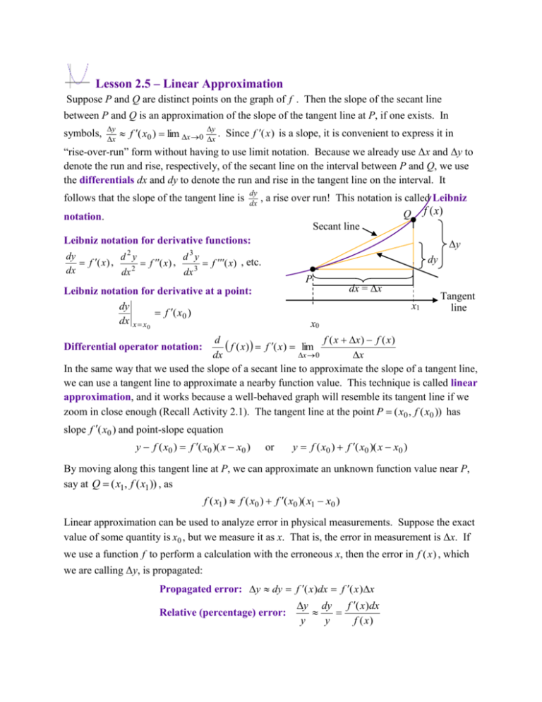
Lesson 2.5 – Linear Approximation
Suppose P and Q are distinct points on the graph of f . Then the slope of the secant line
between P and Q is an approximation of the slope of the tangent line at P, if one exists. In
symbols,
y
x
 f ( x0 )  lim x 0
y
x
. Since f (x ) is a slope, it is convenient to express it in
“rise-over-run” form without having to use limit notation. Because we already use Δx and Δy to
denote the run and rise, respectively, of the secant line on the interval between P and Q, we use
the differentials dx and dy to denote the run and rise in the tangent line on the interval. It
follows that the slope of the tangent line is
dy
dx
, a rise over run! This notation is called Leibniz
f (x)
Q
notation.
Secant line
Leibniz notation for derivative functions:
2
Δy
3
dy
d y
d y
 f ( x ) ,
 f ( x ) ,
 f ( x ) , etc.
2
dx
dx
dx 3
dy
P
Leibniz notation for derivative at a point:
dy
 f ( x0 )
dx x  x 0
dx = Δx
x1
Tangent
line
x0
d
 f ( x )   f ( x )  lim f ( x  x )  f ( x )
x  0
dx
x
In the same way that we used the slope of a secant line to approximate the slope of a tangent line,
we can use a tangent line to approximate a nearby function value. This technique is called linear
approximation, and it works because a well-behaved graph will resemble its tangent line if we
zoom in close enough (Recall Activity 2.1). The tangent line at the point P  ( x0 , f ( x0 )) has
Differential operator notation:
slope f ( x0 ) and point-slope equation
y  f ( x0 )  f ( x0 )( x  x0 )
or
y  f ( x0 )  f ( x0 )( x  x0 )
By moving along this tangent line at P, we can approximate an unknown function value near P,
say at Q  ( x1, f ( x1 )) , as
f ( x1 )  f ( x0 )  f ( x0 )( x1  x0 )
Linear approximation can be used to analyze error in physical measurements. Suppose the exact
value of some quantity is x 0 , but we measure it as x. That is, the error in measurement is Δx. If
we use a function f to perform a calculation with the erroneous x, then the error in f ( x ) , which
we are calling Δy, is propagated:
Propagated error: y  dy  f ( x )dx  f ( x )x
Relative (percentage) error:
y dy f ( x )dx


y
y
f ( x)